Time to contact; optical tau, т

When xe >> 1 (or x >> z), we can simplify eqns 8.1 and 8.3 to the form

(8.5)

The ratio of distance to velocity is the instantaneous time to reach the viewpoint, which we designate as т (t),

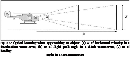
This temporal optical variable is considered to be important in flight control. A clear requirement for pilots to maintain safe flight is that they are able to predict the future trajectory of their aircraft far enough ahead so that they can stop, turn or climb to avoid a hazard or follow a required track. This requirement can be interpreted in terms of the pilot’s ability to detect motion ahead of the aircraft. In his explorations of temporal optical variables in nature (Refs 8.23-8.28), David Lee makes the fundamental point that an animal’s ability to determine the time to pass or contact an obstacle or piece of ground does not depend on explicit knowledge of the size of the obstacle, its distance away or relative velocity. The ratio of the size to rate of growth of the image of an obstacle on the pilot’s retina is equal to the ratio of distance to rate of closure, as conceptualized in Fig. 8.12, and given in angular form by eqn 8.7.

apply computations on the more primitive variables of distance or speed, thus avoiding the associated lags and noise contamination. The time-to-contact information can read­ily be body scaled in terms of eye-heights, using a combination of surface and obstacle т (t)’s, thus affording animals with knowledge of, for example, obstacle heights relative to themselves.

While making these assertions, it is recognized that much spatial information is available to a pilot and will provide critical cues to position and orientation and perhaps even motion. For example, familiar objects clearly provide a scale reference and can guide a pilot’s judgement about clearances or manoeuvre options. However, the temporal view of motion perception purports that the spatial information is not essential to the primitive, instinctive processes involved in the control of motion.

Tau research has led to an improved understanding of how animals and humans control their motion and humans control vehicles. A particular interest is how a driver or pilot might use т to avoid a crash state, or how т might help animals alight on objects. A driver approaching an obstacle needs to apply a braking (deceleration) strategy that will avoid collision. One collision-avoid strategy is to control directly the rate of change of optical tau, which can be written in terms of the instantaneous distance to stop (x), velocity (x) and acceleration (x) in the form:

xx

т = 1 – -^ (8.8)

x2

The system used here for defining the kinematics of motion is based on a negative gap x being closed. Hence, with x < 0 and x > 0, т > 1 implies accelerating flight, т = 1 implies constant velocity and т<1 corresponds to deceleration. In the special case of a constant deceleration, the stopping distance from a velocity x is given by

Hence, a decelerating helicopter will stop short of the intended hover point if at any point in the manoeuvre

-x2

2x

Using eqns 8.7 and 8.8, this condition can be written more concisely as

dr

— < 0.5 (8.11)

dt

A constant deceleration results in Г progressively decreasing with time and the pilot stopping short of the obstacle, unless Г = 0.5 when the pilotjust reaches the destination.

The hypothesis that optical r and Г are the variables that evolution has provided the animal world with to detect and rapidly process visual information, suggests that these should be key variables in flight guidance. In Ref. 8.26, Lee extends the concept to the control of rotations, related to how athletes ensure that they land on their feet after a somersault. For helicopter manoeuvring, this can be applied to control in turns, connecting with the heading component of flight motion, or in vertical manoeuvres, with the flight path angle component of the motion. For example, with heading angle ф and turn rate ф, we can write angular r as

ф

r (t) = у (8.12)

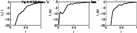
A combination of angular and translational r ’s, associated with physical gaps, needs to be successfully picked up by pilots to ensure flight safety. Figure 8.13 illustrates three examples of motion r variations as a function of normalized manoeuvre time. The results are derived from flight simulation tests undertaken on the Liverpool Flight Simulator in, nominally, good visual conditions. In all three cases the final stages of the manoeuvre (t approaches 1) are characterized by a roughly constant Г, implying, as noted above, a constant deceleration to the goal.

Reaching a goal with a constant Г can be achieved without a constant deceleration of course, and we shall see later in this chapter what the different deceleration profiles look like. For example, if the maximum deceleration towards the goal occurs late in the manoeuvre, then 0.5 <T < 1.0, while an earlier peak deceleration corresponds to 0.0 < Г < 0.5. An interesting case occurs when Г = 0, so that however close to the goal r remains a constant c, i. e.,

x

r = – = c (8.13)

x

The only motion that satisfies this relationship is an exponential one, with the goal approached asymptotically.

An interesting discovery of r control, although unbeknown at the time, is de­scribed in Ref. 8.29. In the early 1970s, researchers at NASA Langley conducted flight

0

400 800 1200 1600 2000 2400 2800 ft

1 l___________ l___________ l___________ l___________ l____________ l___________ l

Range

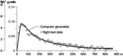
Fig. 8.14 Deceleration profile for helicopter descending to a landing pad (from Ref. 8.29)

trials using several different helicopter types in support of the development of instru­ment flight procedures and the design of flight director displays to aid pilots during the approach and landing phases in poor visibility conditions. The engineers had pos­tulated particular deceleration profiles as functions of height and distance from the landing zone, and the pilots were asked to evaluate the systems based on workload and performance. Several different design philosophies were evaluated and the pilots commented that none felt intuitive and that they would use different control strategies in manual landings, particularly during the final stages of the approach. The linear deceleration profiles resulted in pilots concerned that they were being commanded to hover well short of the touchdown point. The constant deceleration profile was equally undesirable and led to a high pitch/low power condition as the hover was approached. The pilots were asked to fly the approaches manually in good visual conditions, from which the deceleration profiles would be derived and then used to drive the flight di­rector. Figure 8.14 shows a typical variation of deceleration during the approach with 50 knots initial velocity at 500 ft above the ground.

Also shown in the figure is the computer-generated profile showing a gradual reduction in speed until the peak deceleration of about 0.15 g is reached 70 m from the landing pad. The ‘computer-generated’ relationship between acceleration, velocity and distance took the form

where k is a constant derived from the initial conditions. Recalling the formulae for т in eqn 8.8, the relationship given by eqn 8.14 can be written in the form

1 – t = kx1-n (8.15)

The parameters k and n were computed as constants in any single deceleration but varied with initial condition and across the different pilots. The range power parameter

n varied between 1.2 and 1.7. Note that a value of unity corresponds to a constant t for the whole manoeuvre. Equation 8.15 suggests that, at long range, the pilot is maintaining constant velocity (t=1), consistent, of course, with the steady initial flight

і

condition. As range is reduced, т reduces until x = kn-1 when т = 0 and the approach becomes exponential. Beyond this, the representation in eqn 8.15 breaks down, as it predicts a negative т, i. e., the helicopter backs away from the landing pad, although this can happen in practice. Approaches at constant т may seem ineffective because the goal is never reached, but there is evidence that pilots sometimes use this strategy during the landing flare in fixed-wing aircraft, perhaps as a ‘holding’ strategy as the flight path lines up with the desired trajectory (see Ref. 8.30).

The concept of t in motion control has significance for helicopter flight in de­graded visual conditions. If the critical issue for sufficiency of visual cues is that they afford the information to allow the pilot to pick up т ’s of objects and surfaces, then it follows that the т ’s are measures of spatial awareness. It would also follow that they would be appropriate measures to use to judge the quality of artificial vision aids and form the underlying basis for the design and the information content of vision aids. This author has conducted a number of experiments to address the question – how do pilots know when to stop, or to turn or pull up to avoid collision? In the following sections some results from this research will be presented.