Tau-Coupling – a paradigm for safety in action

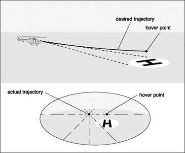
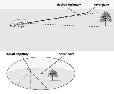
General t theory hypothesizes that the closure of any motion gap is guided by sensing and adjusting the t of the associated physical gap (Ref. 8.24). The theory reinforces the evidence presented in the previous section that information solely about Tx is sufficient to enable the gap x to be closed in a controlled manner, as when making a gentle landing or coming to hover next to an obstacle. According to the theory, and contrary to what might be expected, information about the distance to the landing surface or about the speed and deceleration of approach is not necessary for precise control of the approach and landing. The theory further suggests that a pilot might perceive t of a motion gap by virtue of its proportionality to the t of a gap in a ‘sensory flow-field’ within the visual perception system. In helicopter flight dynamics, the example of decelerating a helicopter to hover over a landing point on the ground serves to illustrate the point. The t of the gap in the optic flow-field between the image of the landing point and the centre of optical outflow (which specifies the instantaneous direction of travel, see Fig. 8.4) is equal to the t of the motion gap between the pilot and the vertical plane through the landing point. This is always so, despite the actual sizes of the optical and motion gaps being quite different; the same applies to stopping at a point adjacent to an obstacle – see Fig. 8.20.

Often movements have to be rapidly coordinated, as when simultaneously making a turn and decelerating to stop, or descending and stopping, or performing a bob-up

Fig. 8.20 г gaps for a helicopter approaching a hover (from Ref. 8.31)

and, simultaneously, a 90° turn. This requires accurate synchronizing and sequencing of the closure of different gaps. To achieve this, visual cues have to be picked up rapidly and continuously and used to guide the action. т theory shows how such closed-loop control might be accomplished by keeping the т ’s of gaps in constant ratio during the movement, i. e., by т-coupling. Evidence of т-coupling in nature is presented in Refs 8.27 and 8.28 for experiments with echo-locating bats landing on a perch and infants feeding. In the present context, if a helicopter pilot, descending (along z) and decelerating (along x ), follows the т – coupling law

тл = ^z (8.16)

then the desired height will automatically be attained just as the aircraft comes to a stop at the landing pad. The kinematics of the motion can be regulated by appropriate choice of the value of the coupling constant k. There is evidence that such coupling can be exploited successfully in vision aids. For example, the system reported in Ref. 8.22 functioned on the principle of the matching of a cluster of forward-directed light beams with different look-ahead distances, which translated into times at a given speed. Such a system was designed as an aid in situations where the natural optical flow was obscured.

In many manoeuvres such as a hover turn or bob-up, there is essentially only one gap to be closed, yet the feedback actions must in principle be similar, whether there are two coupled motion gaps or just one. When a pilot is able to perceive the motion gaps associated with both the displacement and velocity, then т-coupling takes a special form,

with

Tx = k тх (8.18)

Combining eqns 8.17 and 8.18, we can write

Tx = 1 – ^ = 1 – k (8.19)

x2

Hence, the т constant strategy can be expressed as the pilot maintaining the т ’s of the displacement and velocity in a constant ratio. The more general hypothesis is that the closure of a single motion gap is controlled by keeping the т of the motion gap coupled onto what has been described as an intrinsically generated т guide, Tg (Ref. 8.24). One form of such a guide is a constant deceleration motion, from an initial condition xgo(<0), Vgo (>0) given by (c < 0)

c 2

ag = c, vg = vg0 + ct, xg = xg0 + vg01 +-12 (8.20)

At t = T, the manoeuvre duration, we can write

Substitution into the kinematic relationships in eqn 8.20 results in

The constant deceleration т guide has a T = 0.5, a result obtained earlier in this section, and coupling onto this guide with coupling constant к implies

For motions that start at rest, Vg = 0, and end at rest, we need to find a different form of guide. In Ref. 8.24, Lee argues that for natural motions such as reaching, which involve simple phases of acceleration followed by deceleration, it is reasonable to hypothesize that a simple form of intrinsic т guide will have evolved that is adequate for guiding such fundamental movements. In the context of helicopter NoE flight, any of the classic hover-to-hover repositioning manoeuvres fit into this category of motions. Indeed, in any manoeuvre that takes the aircraft from one state to another, the pilot is, in essence, closing a gap of one kind or another. The hypothesized intrinsic tau guide corresponds to a time-varying quantity, perhaps a triggered pattern within the perception system, which changes from one state to another with a constant acceleration. Surprisingly, coupling onto this ‘constant acceleration’ intrinsic guide does not, however, generate a motion of constant acceleration. The resultant motion is, rather, one with an accelerating phase followed by a decelerating phase. From a similar analyses to the case of the constant deceleration guide, the equations describing the changing Tg can be derived and written in the form

where T is the duration of the aircraft or body movement and t is the time from the start of the movement. Coupling the т of a motion gap, Tx, onto such an intrinsic tauguide, Tg, is then described by the equation

Tx = kTg (8.25)

for some coupling constant k. The intrinsic tau guide, Tg, has a single adjustable parameter, T, i. e., its duration. The value of T is assumed to be set to fit the movement either into a defined temporal structure, as when coming to a stop in a confined space, or in a relatively free way, as in the simple movement of reaching for an object. In the case of a helicopter flying from hover to hover across a clearing, we can hypothesize that time constraints are mission related and the pilot can adjust the urgency, within limits, through the level of aggressiveness applied to the controls. The kinematics of a movement can be regulated by setting both T and the coupling constant, к in eqn 8.18, to appropriate values. For example, the higher the value of k, the longer will be the acceleration period of the movement, the shorter the deceleration period and the more abruptly will the movement end. We describe situations with к values >0.5 as hard stops (i. e., к close to unity corresponds to a situation where the peak velocity is pushed close to the end of the manoeuvre) and situations with к < 0.5 as soft stops, similar to the constant T strategy.

The following of a constant acceleration guide in an accel-decel manoeuvre is conceptualized in Fig. 8.21. Both aircraft and guide, shown as a ball, start at the same

/с = 0.2

к= 0.3

/с =0.4

/(=0.5

Fig. 8.21 Following a constant acceleration г guide in an accel-decel manoeuvre

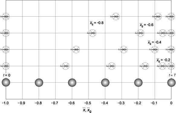
point (normalized distance Xg = —1.0) and time (t = 0) and reach the end of the manoeuvre at the same time, t = T. The ball is continuing to accelerate at this point of course, while the helicopter has come to the hover. For the case к = 0.5, the aircraft has covered about 35% of the manoeuvre distance when Xg = —0.8 and about 85% of the distance when Xg = —0.4. With к = 0.2, when Xg = —0.8, the aircraft has covered two-thirds of the manoeuvre and when Xg = —0.6, the aircraft is within 10% of the stopping point. As к increases, so does the point in the manoeuvre when the reversal from acceleration to deceleration occurs. The time in the manoeuvre when the reversal occurs, tr, can be derived as a function of the coupling coefficient к by noting that, at this point, tx = 1; from eqns 8.24 and 8.25, we can write

"=2 (■+(2)1=1 (826)

This equation can be rearranged into the form

tr=22—yT (827)

Thus, when к = 0.2, tr = 0.333T, when к = 0.4, tr = 0.5T and when к = 0.6, tr = 0.67T, etc.

When two variables, i. e., the motion x and the motion guide Xg, are related through their t-coupling in the form of eqn 8.25, it can be shown (Ref. 8.23) that they are also related through a power law

x a x]Jк (8.28)

This relationship is ubiquitous in nature, governing the relationships between stimuli and sensory responses. Normalizing the distance and time by the manoeuvre length and duration respectively, the motion kinematics (for negative initial x) can be written

as

The coupling parameter к determines exactly how the closed-loop control func­tions, e. g., proportional as к approaches 1 or according to a square law when к = 0.5. The manoeuvre kinematics are presented in Fig. 8.22 of a motion that perfectly tracks the constant acceleration t guide for various values of coupling constant к. The mo­tion t is shown in Fig. 8.22(a), the motion gap, X, in Fig. 8.22(b), the gap closure rate (normalized velocity) in Fig. 8.22(c) and the normalized acceleration in Fig. 8.22(d); all are shown plotted against normalized time.

The closure rate, shown in Fig. 8.22(c), illustrates a typical accel-decel-type velocity profile (cf. X in Fig. 8.16). For к = 0.2 the maximum velocity occurs about 30% into the manoeuvre, while for к = 0. 8 the peak occurs close to the end of the

manoeuvre.

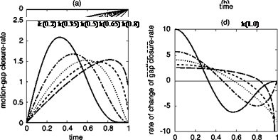Fig. 8.22 Profiles of motions following the constant acceleration guide

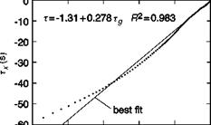
An example of the success of this more general strategy is shown in Fig. 8.23, showing the same case from Ref. 8.31, illustrated previously in Fig. 8.16, but now for the helicopter flying the complete accel-decel manoeuvre. The coupling coefficient is 0.28, giving a power factor of 3.5, with a correlation coefficient of 0.98.

In the analysis of the Ref. 8.31 data, the start and end of the manoeuvres were cropped at 10% of the peak velocity. The tests were flown on the DERA/QinetiQ large motion simulator as part of a series of tests with a Lynx-like helicopter examining the effect of levels of aggressiveness on handling qualities and simulation fidelity. Considering all 15 accel-decels that were flown, the mean values of k follow the trends expected based on Fig. 8.22 (low aggression, k = 0.381; moderate aggression, k = 0.324; high aggression, k = 0.317). As the aggression level increases, the pilot elects to initiate the deceleration earlier in the manoeuvre: low aggression 0.5T into manoeuvre when т ~ 6 s; high aggression 0.4T into manoeuvre when т ~ 4.5 s. The pilot is more constrained during the deceleration phase, with the pilot limiting the nose-up attitude to about 20° to avoid a complete loss of visual cues in the vertical field of view.

0

-60

An intrinsic t guide is effectively a mental model, created by the nervous system, which directs the motion. It clearly has to be well informed (by visual cues in the present case) to be safe. Constant acceleration is one of the few natural motions, created in the short term by the gravitational field, so it is not surprising that the perception system might well have developed to exploit such motions. But the nature of the coupling, the chosen manoeuvre time T and profile parameter к must depend on the performance capability of the aircraft (or the animal performing a purposeful action), and pilots (or birds) need to train to ‘programme’ these patterns into their repertoire of flying skills. When the visual environment degrades so does the ability of the pilot’s perception system to pick up the required information and hence to track the error between actual motions and intrinsic guides. The UCE is, in a sense, a measure of this ability, suggesting that there should be a relationship between UCE and the t of the motion when initiating a manoeuvre to stop, turn or pull-up. In the low-aggression case of Ref. 8.31, the pilot returned Level 1 HQRs and initiated the deceleration when t ~ 6 s, taking about 10 s to come to the hover. The pilot could clearly pick up the visual ‘cues’ of the trees at the stopping point throughout.

The question of how far, or more appropriately how long, into the future the pilot needs to be able to see is critical to flight safety and the design of vision augmentation systems. The research reported in Ref. 8.31 has been extended to address this question specifically, and preliminary results are reported in Ref. 8.33. The focus of attention in this study was terrain following in the presence of degraded visibility, in particular fog, and we continue this chapter with a review of the results of this work and analysis of low-speed terrain following in the DVE.