Our heavyweight helicopter equal in the world does not have
In Rostov started production of the most load-lifting rotary-wing car The Russian holding «Helicopt[...]

Everything about aircrafts and helicopters. News and events in aviation worldwide. Civil, transportation, military helicopters and airplanes.

Everything about aircrafts and helicopters. News and events in aviation worldwide. Civil, transportation, military helicopters and airplanes.

Everything about aircrafts and helicopters. News and events in aviation worldwide. Civil, transportation, military helicopters and airplanes.

Everything about aircrafts and helicopters. News and events in aviation worldwide. Civil, transportation, military helicopters and airplanes.


It has been found that numerical algorithm described above is capable of reproducing the jet screech phenomenon computationally. The nozzle configuration in the experiment of Ponton and Seiner (1992) is used in the simulation. Figure 15.55 shows the computed density field in the x-r plane at one instance after the initial transient disturbances have propagated out of the computational domain. The screech feedback loop locks itself into a periodic cycle without external interference. As can be seen, sound waves of the screech tones are radiated out in a region around the fourth and fifth shock cell downstream of the nozzle exit. Most of the prominent features of the numerically simulated jet screech phenomenon are in good agreement with physical experiment.
15.6.2.1 
Mean Velocity Profiles and Shock Cell Structure
To demonstrate that numerical simulation can, indeed, reproduce the physical experiment, the accuracy of the computed mean flow velocity profiles of the simulated jet is tested by comparison with experimental measurements. For this purpose, the time-averaged velocity profiles of the axial velocity of a Mach 1.2 cold jet from one jet diameter downstream of the nozzle exit to seven diameters downstream at one diameter intervals are measured from the numerical simulations. They are shown as a function of n* = (r – r05)/x in Figure 15.56, where r05 is the radial distance from the jet axis to the location where the axial velocity is equal to one half of the fully expanded jet velocity. Numerous experiments have shown that the mean velocity profile when plotted as a function of n* would nearly collapse into a single curve. The single curve is well represented by an error function in the following form:
![]() U = 0.5[1 – erf (an*)], Uj
U = 0.5[1 – erf (an*)], Uj
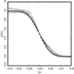 Figure 15.56. Comparison between computed mean velocity profiles at M. = 1.2 and experiment (Lau, 1981). Simulation
results:——– , x/D = 1.0;——– , x/D =
2.0; — • —, x/D = 3.0;———– , x/D =
4.0;——— , x/D = 5.0;—– ,x/D = 6.0;
………… , x/D = 7.0. Experiment U/U. =
0.5[1 – erf(an*)]; o, a = 17.0.
|
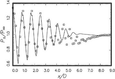
Figure 15.57. Comparison between calculated time-averaged pressure distribution along the centerline of a Mach 1.2 cold jet and the measurement of Norum and Brown (1993).- , simulation; □, experiment. |
where a is the spreading parameter and Uj is the fully expanded jet exit velocity. Extensive jet mean velocity data had been measured by Lau (1981). By interpolating the data of Lau to Mach 1.2, it is found that experimentally a is nearly equal to 17.0. The empirical formula with a = 17.0 is also plotted in Figure 15.56 (the circles). It is clear that there is good agreement between measured mean velocity profile and those of the numerical simulation.
One important component of the screech feedback loop is the shock cell structure inside the jet plume. To ensure that the simulated shock cells are the same as those in an actual experiment, the time-averaged pressure distribution along the centerline of the simulated jet at Mach 1.2 is compared with the experimental measurements of Norum and Brown (1993). Figure 15.57 is a plot of the simulated and measured pressure distribution as a function of downstream distance. It is clear from this figure that the first five shocks of the simulation are in good agreement with experimental measurements both in terms of shock cell spacing and amplitude. Beyond the fifth shock cell, the agreement is less good. However, it is known that screech tones are generated around the fourth shock cell. Therefore, any minor discrepancies downstream of the fifth shock cell would not invalidate the screech tone simulation.