T on the rising curve

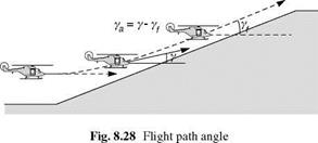
For the t analysis, the aircraft flight path angle у is converted to ya, the negative perturbation in у from the final state, as illustrated in Fig. 8.28.

If the aircraft’s normal velocity w is small relative to the forward velocity V, the flight path angle can be approximated as

w

Y *-y (8.35)

If the final flight path angle is yf, then the y-to-go, Ya can be written as

Ya = Y – Y f

x (m)

Fig. 8.26 Distance to the slope surface (in meters and eye-heights)

* (m)

Fig. 8.27 Times to the slope surface (t to surface)

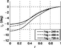
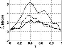
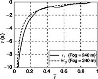
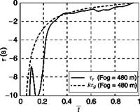
Fig. 8.29 ya, ya during the climb

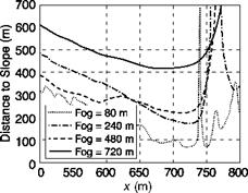
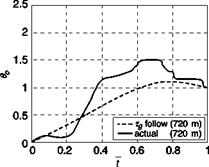
The y’s-to-go and associated time rates of change are plotted in Fig. 8.29 for the UCE = 1 and UCE = 2 fog-line cases, although it should be noted that the 240-m case is actually borderline UCE = 2/UCE = 3. In Fig. 8.29, time has been normalized by the duration of the climb transient (fog = 240 m, T = 2.5 s; fog = 480 m, T = 4.3 s; fog = 720 m, T = 4.7 s). The final value of the flight path angle was chosen as the value when Y first became zero (thus defining T and yf); hence, although the hill had a 5° slope, the values used correspond to the first overshoot peak value. From that time on, the pilot closes the loop on a new т gap, related to the flight path error from above. As can be seen from the initial conditions, the pilot tends to overshoot the 5° hill slope with increasing extent as the UCE degrades – flight path angle of 8.5° for the 240-m fog-line (UCE 2/3), 7° for the 480-m fog-line case (UCE 2) and 6° for the 720-m case (UCE 1).

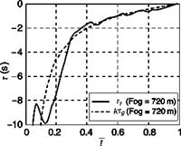
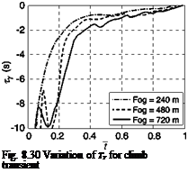
Figure 8.30 shows the variation of Ty with normalized time. The fluctuations reflect the higher frequency content in the Y function. As the goal is approached the curves straighten out and develop a slope of between 0.6 and 0.7, corresponding to the pilot following the т constant guide with peak deceleration close to the goal.

As with the accel-decel manoeuvre, the pilot is changing from one state to an­other (horizontal position for the accel-decel, flight path angle for the climb), and as discussed earlier, the natural guide for ensuring that such changes of state are achieved successfully is the constant acceleration guide, with the relationship, Ty = кTg.

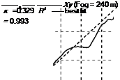
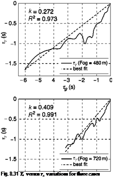
Figure 8.31 shows results for the Ty versus Tg correlation for the terrain climb in the three fog conditions. In the UCE = 1 case (720 m fog), apart from a slight departure at the end of the manoeuvre, the fit is tight for the full 5 s (R2 = 0.99). The departures from the close fit at both the beginning and end of such state change

manoeuvres are considered to be transient effects, partly due to the need for the pilot to ‘organize’ the visual information so that the required gaps are clearly perceived and partly due to the contaminating effects of the pitch changes that disrupt the visual cues for flight path changes picked up from the optic flow. Table 8.3 gives the coupling coefficients, k, for all cases flown. The lower the k value, the earlier in the manoeuvre the maximum motion gap closure rate occurs (e. g., a value of 0.5 corresponds to a symmetric manoeuvre). There is a suggestion that k reduces as UCE degrades, confirmed by the results in Fig. 8.31. The pilot has commanded a flight path angle rate of about 6°/s less than 40% into the manoeuvre in the UCE = 2-3 case compared with about 2.5°/s about 50% into the manoeuvre in the UCE = 1 case.

Typical correlations between xy and Tg are shown in Fig. 8.32, plotted against normalized time. The relatively constant slope during the second half of the manoeuvre indicates that the pilot has adopted a constant T strategy. As expected, the test data track the constant acceleration guide fairly closely over the whole manoeuvre.

The results reveal a strong level of coupling with the T guide. This was not unexpected. In a complementary study, t analysis has been conducted on data from approach and landing manoeuvres for fixed-wing aircraft (Ref. 8.30). During the land­ing flare, the pilot follows the T guide to the touchdown. Instrument approaches where the visibility was reduced to the equivalent of Cat IIIb (cloud base 50 ft, runway visual range 150 ft) were investigated, and in some cases the coupling reached the limiting case of constant t, the pilot effectively levelling off just above the runway. The results presented are consistent with those presented in Ref. 8.30, unsurprisingly as the flare and terrain climb tasks make very similar demands on the pilot in terms of visual information.

From eqns 8.34 and 8.35, we can write the equation for flight path perturbation dynamics as

with

Ya (t = 0) = – Yf

-6 -5 -4 -3 -2 -1 О

Tg(s)

-6 -5 4 -3 -2 -1 О

*(s)

Table 8.3 Correlation constants and fit coefficients – following the constant acceleration guide Case k R2 Fog = 720 m (run 1) 0.3930 0.9820 Fog = 720 m (run 2) 0.3490 0.9130 Fog = 720 m (run 3) 0.4090 0.9910 Fog = 480 m (run 1) 0.2720 0.9730 Fog = 480 m (run 2) 0.3670 0.9960 Fog = 240 m (run 1) 0.3490 0.9960 Fog = 240 m (run 2) 0.2060 0.8850 Fog = 240 m (run 3) 0.3290 0.9930

Fig. 8.32 Correlation between times to close the flight path gap for the motion and guides

1

(8.39)

w

where

(8.40)

The instantaneous time to reach the goal of у = уf is defined as

Ty a = — (8.41)

Ya

Following a t guide such that tx = kTg results in motion that follows the guided motion as a power law

x = Cxg1 к (8.42)

where C is a constant.

Recapping from earlier in the chapter, the constant acceleration guide has the forms given by

agis the constant acceleration of the guide. As discussed earlier and shown in Fig. 8.21, the motion begins and ends hand-in-hand with the guide, but initially overtakes before being caught up and passed by the guide at the goal.

The equations for the flight path motion and its derivatives can then be developed (see Ref. 8.24) and written in the normalized form

Ya = ? a -12)( 1 -1)

From eqn 8.39, the collective control can then be written in the general form в 0 = 1 + ta Y a + Y a

Combining with eqns 8.45 and 8.46, the normalized collective pitch is given by the expressions

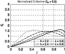
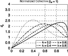
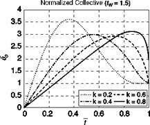
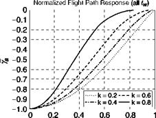
The normalized functions в0 and Ya(independent of tw ) are plotted in Figs 8.33 and 8.34, as a function of normalized time for different values of coupling constant k. The three cases correspond to the parameter tw set at 0.5,1.0 and 1.5. The strategy involves increasing the collective gradually, and well beyond the steady-state value, and then decreasing as the target rate of climb is approached. For tw = 0.5, when the heave time constant is half the manoeuvre duration, the overdriving of the control is limited to about 50% of the steady-state value. As the ratio increases to 1.5, so too does the overdriving to as much as 250% at the lower k values. This overshoot is unlikely to be achievable even when operating with a low-power margin. As k increases, the peak

Fig. 8.33 Normalized collective pitch for a flight path angle change following a constant acceleration т guide – variations with k and tw

collective lever position occurs later in the manoeuvre until the limiting case where it is reduced as a down-step in the final instant to bring Ya to zero. When approaching a slope, the pilot has scope to select T, hence tw, and k, to ensure that the control and hence the manoeuvre trajectory are within the capability of the aircraft. Whatever values are selected, the control strategy is far removed from the abrupt, open-loop character associated with a step input.

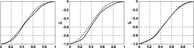
t Fig. 8.34 Normalized flight path response for a flight path angle change following a constant acceleration т guide-variations with k

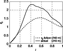
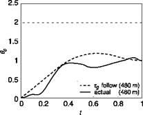
A comparison of normalized collective inputs and flight path angles with the т-coupled predictions for representative cases is shown in Fig. 8.35. The large peak for the 240-m fog-line case resulted in the overshoot to 10° flight path angle discussed earlier and could be argued in a case where the pilot has lost track of the cues that enable the т – coupling to remain coherent. The actual pilot control inputs appear more abrupt than the predicted values but it again could be argued that the pilot needs to stimulate the flow-field initially with such inputs. There is good agreement for the flight path angle variations.

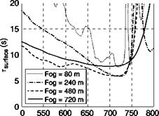
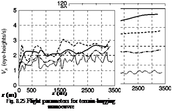
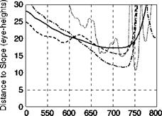
In Ref. 8.31, the notion was put forward that ‘the overall pilot’s goal is to overlay the optic flow-field over the required flight trajectory – the chosen path between the trees, over the hill or through the valley – thus matching the optical and required flight motion’. This concept can be extended to embrace the idea that the overlay technique can happen within a temporal as well as spatial context. The results presented above convey a compelling impression of pilots coupling onto a natural т guide during the 3-5 s of the climb phase of the terrain-hugging manoeuvre. As in the accel-decel manoeuvre, pilots appear to pick up their visual information from about 12 to 16 eye – heights ahead of the aircraft and establish a flight speed that gives a corresponding look-ahead time of about 6-8 s. As height is reduced, the pilot slows down to maintain velocity in eye-heights, and corresponding look-ahead time, relatively constant. The manoeuvre is typically initiated when the Tsurface reduces to about 6 s and takes between 4 and 5 s to complete. Of course, the manoeuvre time must depend on the heave time constant of the aircraft being flown. For the FLIGHTLAB Generic Rotorcraft simula­tion model used in the trials, tw varies between 3 s in hover and 1.3 s at 60 knots, reducing to below 1 s above 100 knots. Much stronger interference between the aircraft and task dynamics would be expected with aircraft that exhibited much slower heave response (e. g., aircraft featuring rotors with high-disc loadings), as illustrated in Fig. 8.32.

The temporal framework of flight control offers the potential for developing more quantitative UCE metrics. For example, in the terrain manoeuvres described above, the UCE = 3 case was characterized by the distance to visual obscuration coming within about 20% of the 12 eye-height point (i. e., ~ 1 s). For the UCE = 1 case, the margin was more than 6 s. Sufficiency of visual information for the task is the essence of safe flight and т envelopes can be imagined which relate to the terrain contouring and

t	t
Fig. 8.35 Comparisons of normalized pilot control activity and flight path with r-following strategy

associated MTEs. These constructs might then be used to define the appropriate speed and height to be flown in given terrain and visual environment. Visual information that provides clear cues to the pilot to enable coupling onto the natural т guides could then form the basis for quantitative requirements for artificial aids to visual guidance that improve both attitude and translational rate contributions to the UCE.

The goal of a pilotage augmentation system, designed to extend operational ca­pability in a DVE, must be to achieve performance without compromising safety, reducing fatigue by reducing cognitive workload and increasing confidence to allow aggressive manoeuvring. The designers of such synthetic vision systems can utilize the natural, reflexive pilot skills, and several pathway-in-the-sky type formats are currently under development or being explored in research (e. g., Refs 8.34, 8.35) that exhibit such properties. Designers also have the freedom to combine such formats with more detailed display structures for precision tracking, e. g., the pad-capture mode on the AH-64A (Ref. 8.36). This type of format requires the pilot to apply cognitive atten­tion, closing the control loop using detailed individual features to achieve the desired precision, hence risking a loss of situation awareness with respect to the outside world. Achieving a balance between precision and situation awareness is the pilot’s task and what is appropriate will change with different circumstances. Quite generally however, when equipped with an adequate sensor suite, there seems no good reason why a large part of the stabilization and tracking tasks should not be accomplished by the automatic flight control system.

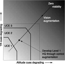
Improving flying qualities for flight in a DVE is about the integration of vision and control augmentation. The UCE describes the utility and adequacy of visual cues for guidance and stabilization. The pilot rates the visual cues based on how aggressively and precisely corrections to attitude and velocity can be made. An assumption in this approach is that the aircraft has Level 1, rate command handling qualities in a GVE. In a DVE, the handling qualities of the aircraft degrade because of the impoverishment

Fig. 8.36 Conceptualization of flying qualities improvements in the DVE

of the visual cues. According to the UCE methodology of ADS-33, provided the DVE is no worse than UCE = 3, Level 1 handling qualities can be ‘recovered’ by control augmentation. The augmentation process therefore appears straightforward, at least in principle: recover to UCE = 3 or better via vision augmentation, and then use control augmentation, to recover Level 1 flying qualities – Fig. 8.36 conceptualizes this idea.

Helicopter flight in degraded visibility will remain dangerous, with a consequent higher risk to flight safety, without vision augmentation. A key characteristic of a good vision aid is that it should provide the pilot with clear and coherent cues for judging operationally relevant, desired and adequate performance standards for flight path and attitude control. The ADS-33 handling qualities requirements then provide the design criteria for control augmentation. The higher the levels of augmentation and the stronger the control feedback gains, required an increased level of safety monitoring and redundancy to protect against the negative effects of failure, which leads us to the second topic in this chapter.