Sample Computer Programs

Three sample programs are provided in this appendix. The first set of programs is for solving the one-dimensional convective wave equation. There are two programs. The first program uses the DRP scheme. The second program uses the standard 2nd, 4th and 6th order central difference scheme for spatial discretization and the Runge-Kutta scheme for time marching. The second set of programs is for solving the linearized two-dimensional Euler equations. The DRP scheme is used. The third set of programs is for solving the non-linear three-dimensional Euler equations. The DRP scheme is used.

G.1 Sample Program for Solving the One-Dimensional Convective Wave Equation

The numerical solution to the following problem in an infinite domain is considered. The convective equation in dimensionless form is

d u d u

+ = 0 91 dx

Two types of initial conditions are used in this example

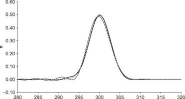
1. A Gaussian function.

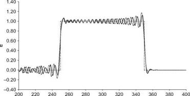
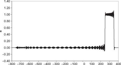
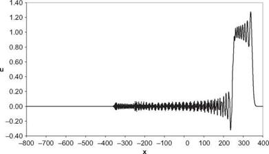
2. A box car function i. e.,

u(x, 0) = H(x + L) – H(x – L) where H (x) is the unit step function.

The Fortran 90 program below computes the solution using the DRP scheme.

program DRP_1D

This code solves the 1-D convective wave equation on the real line using the DRP scheme

-equation is non-dimensionalized by mesh spacing and wave speed

-equation is discretized with 7-point spatial stencils and 4 level multi-step time advancement

-the solution is advanced from the initial conditions to the desired time and then output to file

Variables:

id – number of mesh points to the left and right of origin nmax – maximum number of time steps t – time

delt – time step u – solution values

k – time derivatives, dudt, at different time levels

kl – converts time level to index in k array a – spatial stencil coefficients

b – multi-step advancement coefficients

implicit none

integer, parameter::rkind=8,id=800 integer::n, l,nmax, bh integer, dimension(-3:0)::kl real(kind=rkind)::delt, h,t real(kind=rkind), dimension(-id-3:id+3)::u real(kind=rkind), dimension(-3:0,-id:id)::k real(kind=rkind), dimension(-3:3)::a real(kind=rkind), dimension(-3:0)::b integer::outdata=20 !

! Open output data file ‘out. dat’

!

open(unit=outdata, file="outDRP. dat", status="replace") !

! Optimized 7-point spatial stencil

!

a(-3)=-0.02003774846106832_rkind

a(-2)=0.163484327177606692_rkind

a(-1)=-0.766855408972008323_rkind

a(0)=0.0_rkind

a(1)=0.766855408972008323_rkind

a(2)=-0.163484327177606692_rkind

a(3)=0.02003774846106832_rkind

!

! Optimized multi-step

!

b(0)=2.3025580888_rkind

b(-1)=-2.4910075998_rkind

b(-2)=1.5743409332_rkind

b(-3)=-0.3858914222_rkind

I

! Set simulation parameters I

delt=0.1_rkind! time step size (stability/accuracy limit is 0.2111) nmax=3000 ! maximum number of time steps I

! Set ‘boundary’ conditions (assume u=0 far from origin)

I

u(-id-3)=0.0_rkind

u(-id-2)=0.0_rkind

u(-id-1)=0.0_rkind

u(id+1)=0.0_rkind

u(id+1)=0.0_rkind

u(id+3)=0.0_rkind

!

! Set initial conditions!

t=0.0_rkind

!

! Gaussian function with half-width ‘bh’ and height ‘h’ !bh=3

!h=0.5_rkind! do l=-id, id

! u(l)=h*exp(-log(2.0_rkind)*(real(l, rkind)/real(bh, rkind))**2) !end do!

! Boxcar

!

u=0.0_rkind

u(-50:50)=1.0_rkind

!

! Set solution to zero for t<0

!

k=0.0_rkind

kl(-3)=-3

kl(-2)=-2

kl(-1)=-1

kl(0)=0

!

!——————————————————————

!

! Main loop – march nmax steps with multi-level DRP

do n=1,nmax!

t=t+delt

write (*,*)"n: ",n," t: ",real(t,4)

!

! Update k

!

do l=-id, id

k(kl(0),l)=a(-3)*u(l-3)+a(-2)*u(l-2)+a(-1)*u(l-1)+a(1)*u(l+1)+a(2)*u(l+2)+a(3)*u(l+3) end do!

! Update u to time level n

!

do l=-id, id

u(l)=u(l)-delt*(b(0)*k(kl(0),l)+b(-1)*k(kl(-1),l)+b(-2)*k(kl(-2),l)+b(-3)*k(kl(-3),l)) end do!

! Shift k array back kl =cshift(kl,1)

end do!

! Output u results !

50 format(i8,e16.7e3) do l=-id, id

write (outdata,50)l, u(l) end do!

stop

end program DRP_1D

The Fortran 90 program below computes the solution to the convective wave equa­tion by means of the standard 2nd, 4th and 6th order central difference scheme for spatial discretization and the Runge-Kutta scheme for time marching.

program RK4_1D

This code solves the 1-D convective wave equation on the real line using the standard fourth order Runge-Kutta scheme – equation is non-dimensionalized by mesh spacing and wave speed

-equation can be discretized with either 6th,4th,2nd order spatial stencils

-the solution is advanced from the initial conditions to the desired time and then output to file

Variables:

id – number of mesh points to the left and right of origin nmax – maximum number of time steps t -time delt – time step

и, ut – solution values

к, k1,k2 – time derivatives, dudt

a2	-2nd	order	spatial	stencil	coefficients
a4	-4th	order	spatial	stencil	coefficients
a6	-6th	order	spatial	stencil	coefficients

implicit none

integer, parameter::rkind=8,id=800 integer::n, l,nmax, bh, iorder real(kind=rkind)::delt, dth, dt6,h, t real(kind=rkind), dimension(-id-3:id+3)::u, ut real(kind=rkind), dimension(-id:id)::k, k1,k2 real(kind=rkind), dimension(-1:1)::a2 real(kind=rkind), dimension(-2:2)::a4 real(kind=rkind), dimension(-3:3)::a6 integer::outdata=20 !

! Open output data file ‘out. dat’

!

open(unit=outdata, file="outRK4.dat", status="replace") !

! 2nd order spatial stencil

!

a2(-1)=-0.5_rkind

a2(0)=0.0_rkind

a2(1)=0.5_rkind

!

! 4th order spatial stencil

!

a4(-2)=1.0_rkind/12.0_rkind

a4(-1)=-2.0_rkind/3.0_rkind

a4(0)=0.0_rkind

a4(1)=2.0_rkind/3.0_rkind

a4(2)=-1.0_rkind/12.0_rkind

6th order stencil

a6(-3)=-1.0_rkind/60.0_rkind

a6(-2)=3.0_rkind/20.0_rkind

a6(-1)=-3.0_rkind/4.0_rkind

a6(0)=0.0_rkind

a6(1)=3.0_rkind/4.0_rkind

a6(2)=-3.0_rkind/20.0_rkind

a6(3)=1.0_rkind/60.0_rkind

!

! Set simulation parameters!

delt=0.4_rkind! time step size

dth=delt*0.5_rkind

dt6=delt/6.0_rkind

nmax=750 ! maximum number of time steps iorder=6 ! order of the spatial stencil (2,4,6)

!

! Set ‘boundary’ conditions (assume u=0 far from origin) !

u(-id-3)=0.0_rkind

u(-id-2)=0.0_rkind

u(-id-1)=0.0_rkind

u(id+1)=0.0_rkind

u(id+1)=0.0_rkind

u(id+3)=0.0_rkind

!

ut=0.0_rkind

!

! Set initial conditions!

t=0.0_rkind

!

! Gaussian function with half-width ‘bh’ and height ‘h’ !bh=3

!h=0.5_rkind! do l=-id, id

! u(l)=h*exp(-log(2.0_rkind)*(real(l, rkind)/real(bh, rkind))**2) !end do!

! Boxcar!

u=0.0_rkind

u(-50:50)=1.0_rkind

Initial du/dt

call dudt(u, k,iorder)

!

!………………………………………………………….

!

! Main loop – march nmax steps in time using RK4 integration!

do n=1,nmax!

t=t+delt

write (*,*)”n: ",n," t: M, real(t,4)

!

! Second step!

do l=-id, id ut(l)=u(l)+dth*k(l) end do

call dudt(ut, k1,iorder)

!

! Third step

!

do l=-id, id ut(l)=u(l)+dth*k1(l) end do

call dudt(ut, k2,iorder)

!

! Fourth step

!

do l=-id, id ut(l)=u(l)+delt*k2(l) k2(l)=k2(l)+k1(l) end do

call dudt(ut, k1,iorder)

!

! Update u

!

do l=-id, id

u(l)=u(l)+dt6*(k(l)+k1(l)+2.0_rkind*k2(l)) end do!

! Update dudt

!

call dudt(u, k,iorder) end do

! Output u results I

50 format(i8,e16.7e3) do l=-id, id

write (outdata,50)l, u(l) end do!

stop

!

contains

!

subroutine dudt(f, kf, iflag) !

!

! Calculate the derivative du/dt=-du/dx of the convectice wave eqn! – iflag is a flag for the spatial stencil (2nd,4th,6th order)

!

!

implicit none

integer, intent(in)::iflag

real(kind=rkind), intent(in), dimension(-id-3:id+3)::f real(kind=rkind), intent(out), dimension(-id:id)::kf integer::l!

select case (iflag) case (2) do l =-id, id

kf(l)=-(a2(-1)*f(l-1)+a2(1)*f(l+1)) end do case (4) do l =-id, id

kf(l)=-(a4(-2)*f(l-2)+a4(-1)*f(l-1)+a4(1)*f(l+1)+a4(2)*f(l+2)) end do case (6) do l =-id, id

kf(l)=-(a6(-3)*f(l-3)+a6(-2)*f(l-2)+a6(-1)*f(l-1)+a6(1)*f(l+1)+a6(2)*f(l+2)+a6(3)*f(l+3)) end do end select!

return

end subroutine dudt !

end program RK4_1D

Samples of computed results and the exact solutions are shown below.

Gaussian, t=300 I—— DRP ——- RK4-6th……… Exact | x

Boxcar, t=300 I—— DRP RK4-6th……………… Exact |

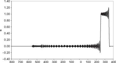
Boxcar, t=300, DRP Scheme x

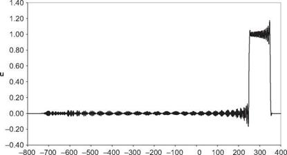
Boxcar, t=300, RK4-2nd

Boxcar, t=300, RK4-6th x

1.1. The governing equation and boundary conditions for a rectangular vibrating membrane of width W and breadth B are

92U 2 / d2Ы d2U

dt2 dx2^~ dy2

At x = 0, x = W, y = 0, y = B, u = 0,

where U is the displacement of the membrane. It is easy to show that the normal mode frequencies of the vibrating membrane are

[2]/2

, where j and к are integers.

Now divide the width into N subdivisions and the breadth into M subdivisions so that Ax = W/N and Ay = B/M. Suppose a second-order central difference is used to approximate the x and y derivatives. This converts the partial differential equation into a partial difference equation, as follows:

[3]

The conditions for E to be a minimum are

[4] For convenience, D(a Ax) may be normalized so that

D (n) = 1. (7.18)

The right side of Eq. (7.14) is a truncated Fourier cosine series. To ensure that D (a Ax) is small when a Ax is small but becomes large when a Ax ^ n, one may use a Gaussian function centered at a Ax = n with half-width a as a template for choosing the Fourier coefficients d. This is done by determining dj such that the integral

[5] There should be no damping for long waves. That is, D (a Ax) ^ 0 as aAx^0. This requires

3

d0 + 2 dj = 0. (7.17)

j=1

7.1. Let us reconsider the initial value problem

9 u d u

+ = 0 9t dx

t = 0, u = H (x + 50) – H (x – 50), where H (x) is the unit step function.

Compute the solution using the 7-point DRP scheme with artificial selective damping. Use a At that satisfies the numerical stability requirement.

[7] Use RA = 0.3, where Ra is the artificial mesh Reynolds number.

[8] Use RA = 0.3/At.

Plot u(x, t) at t = 300 for each case.

7.2. Real fluids have molecular viscosity that tends to damp out long and short wave disturbances. This problem focuses on how best to compute viscous terms to simulate real viscous effects. At the same time, it provides an example illustrating why

[9] Use RA = 3.

[10] 3

— aj ФJ.

Ді j j

j=-3

[11]+dMA)U+A і+(1 – m2 ) 2 ВI=<9-38)

where u(x, y, t) = U(x, y)e-1 ®f.

The second step is to introduce damping into the equation through a so-called complex change of variables. Let о x(x) > 0, о (y) > 0 be the absorption coefficients. The complex change of variables is to let

9.1. Many aeroacoustic problems involve the scattering of vorticity or acoustic waves by an object. To simulate this class of problems in the time domain, the incoming waves are generated by the boundary conditions imposed on the artificial external boundaries of the computation domain.

Dimensionless variables with respect to length scale L (L will be chosen later), velocity scale aTO (ambient sound speed), time scale L/aTO, density scale pTO (ambient density), and pressure scale p^a^ are used. Suppose there is a uniform mean flow

11.1. The optimized extrapolation method can be applied even when the stencil points are not spaced uniformly apart. Let the coordinates of the stencil points be x0, x_1, x_2,…, x__7 (a 7-point stencil). Suppose the extrapolation point is at x = x0 + n. The extrapolation formula is

[14]

f (x0 + n) = Y^ Sjf(x- j )•

j=0

[15]

[16] (R, в, ф, ю)

[17] 0 < r < 0.8