Category Aerodynamic measurements

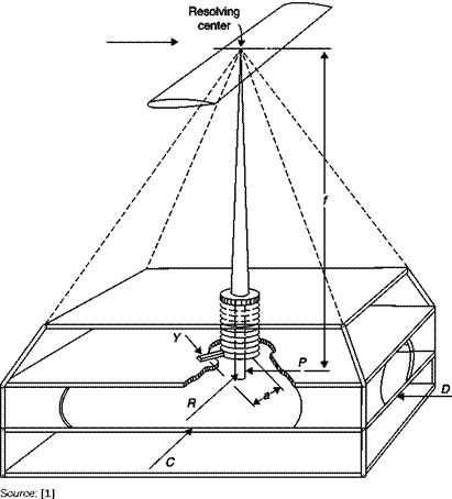Some of the problems of systems with parallel links are eliminated in the pyramidal support (Figure 7.23) where the moments are referred to the center of resolution and the six components are inherently separate and read directly from six units that do not need to add or subtract components. Sensitive issues to be considered in the design and calibration of this type of balance are the perfect alignment of the inclined rods and their deflections. Truncated rods must be carefully aligned so that their extensions pass through a common point. The forces and moments are:

Automatic counterweights balance

Lift = vertical force

Drag = – D Side force = – C Rolling moment = Rf Yawing moment = – Ya Pitching moment = Pf

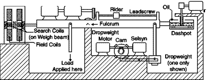
7.3.2.1Dynamometric elements

For each component to be measured manually or automatically (Figure 7.24), balances are used which employ a sliding weight on a worm and cam mechanism to add or remove additional weights. Other types of dynamometers have a load cell, in which the force is balanced by a pressure exerted by a fluid, or strain gages, used more frequently in deformation balances.

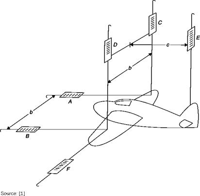
In the schematic of Figure 7.22, the model is supported by wires and forces are measured by 6 dynamometers. The usual components of forces and moments along and around wind axes are calculated, once the weight of the model has been set equal to zero in dynamometers C, D and E, from the equations:

Lift = -(C + D + E)

Drag = A + B Side force = – F Rolling moment = (D – C)b/2 Yawing moment = (A – B)b/2 Pitching moment = – Ec

The balances on parallel links are widely used but the wires have given way to rigid rods such as those in Figure 7.1. They can be built and aligned with minimal difficulty, but have the following disadvantages:

■ the moments are proportional to small differences between large forces, this would adversely affect the precision of the measurement;

Measurement of the aerodynamic force with six dynamometers

■ the center of resolution of forces is not on the model and then the moments are to be transported;

■ drag and lateral force introduce moments of pitch and roll respectively, and these interactions should be removed from the final data;

■ the drag of the supports that protrude from the fairing must be taken into account.

All this makes the following mandatory:

■ a prior calibration of the balance with known weights needed in order to identify the interaction between the various components;

■ measurements taken in a test without a model to determine the drag of the supports (the interference that occurs when model and support are connected remains unknown).

The fundamental difficulty in the design of permanent balances is that they are called upon to measure forces and moments with a high accuracy in the whole range up to the maximum load without appreciable distortions in the structure and down to a small fraction of it. For

example, an experiment on a wing with laminar profile can be followed by tests on a bluff body (such as a radar antenna), and the balance itself should be able to measure the drag of both bodies with sufficient precision. For this reason, permanent balances are designed to have a sensitivity equal to 10-4 of the full scale: in this way also in measured quantities hundred times smaller than the maximum range the accuracy does not fall below 1%. (The same problem occurs with the majority of measuring instruments, but while it is quite normal to provide a laboratory with many pressure gages for different pressure ranges, a wind tunnel is equipped with a single null reading balance, which is therefore “permanent.”)

Usually the balance is mounted outside the test chamber and the connections are made with the model suspended with wires or mounted on rigid struts. In practice, there are not two balances which adopt the same system and a full discussion of all the sophisticated configurations would occupy too much space. Most connections can be classified into two types: parallel links and virtual center.

7.3.1 Classification of balances

The balance is an important tool in a wind tunnel as it allows the direct measurement of the aerodynamic forces acting on the model. Aerodynamic balances are very complex because, unlike balances used to measure weight, they need to measure a force of which are unknown, and variable during the experiment, the direction, the sign and the point of application. In the most general 3D field, it is therefore necessary to measure three forces acting along three axes to find the direction of the aerodynamic force and three torques acting around the same axes to determine the point of application of the force. In the case of 2D motion, it is enough to measure two forces and one moment.

The balances may be classified as:

■ permanent balances: they are part of the wind tunnel and are placed outside the test chamber (Figures 7.1, 7.6 and 7.8); typically one axis is directed in the direction of the axis of the wind tunnel, and hence of the asymptotic velocity, and another is vertical (so the weight of the model affects only one component of the force and one moment);

■ sting balances, dedicated to each model and incorporated into the sting support (Figures 7.2, 7.3, 7.4 and 7.5); an axis generally coincides with the central axis of the model.

Components of the aerodynamic force

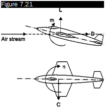D drag C side force r rolling moment m pitching moment n yawing moment

These two systems of axes are respectively the wind axes and the body axes. Usually forces and moments are referred to the wind axis and have the usual names: lift, drag and side force and moments of yaw, roll and pitch (Figure 7.21).

Balances are also classified according to the number of the measured components:

■ one-component balances, able to measure the drag of non-lifting bodies (sphere, cylinder normal to the direction of the velocity and symmetrical airfoils at zero incidence);

■ two-component balances measure lift and drag;

■ three-component balances measure lift, drag and pitching moment;

■ four-component balances measure also the rolling moment;

■ six-component balances give a complete measure of the interaction between body and fluid stream.

Usually, three-component balances are used, sufficient to study sym­metrical flight (side force and roll and yaw moments are zero); only rarely are six-component balances required.

In mechanical balances, the force acting on the model is transmitted through a system of levers through a steel yard along which the weights needed for balancing are slid. In electrical balances, the movements pro­duced by forces cause changes in capacitance, inductance or resistance of an electrical circuit; also quartz transducers are used and, mainly, strain gages.

Depending on the method used for the measurement of the force, balances can be classified as: null reading or deformation balances. In both systems it is necessary for the body to move, even if infinitesimally, in the direction of the applied force:

■ the null reading balances measure the force required to bring the model to the position it had before the application of the aerodynamic force;

■ strain gages balances measure the deformation due to the displacement of the model due to the aerodynamic force.

Both methods can be used with any type of support of the model and in any type of wind tunnel. It is just a historical accident that the null reading method has been associated with the permanent balance, which is typical of the low speeds wind tunnels, while the deformation balances were associated with a sting support, mandatory in supersonic wind tunnels.

■ The advantages of permanent balances are the fact that when the measure is made, the model is again in the initial state, the high resolution, the ability to maintain calibration over long periods of time. The disadvantages are the high cost and the time required for the initial alignment and calibration.

■ The advantages of a sting balance are that the initial cost is lower, though this can be offset by the necessity of having to build many balances with different measuring ranges to suit different needs, and that tests are allowed at very high angles of attack. The disadvantage is the fact that the relationship between displacement and applied force must be determined by calibration and can also be nonlinear, and that at the moment of the measurement the model has shifted from its original position.

No balance can be used for all tests on all possible models, but a permanent balance is more versatile, thanks to the width of the measurement range and the adaptability to unforeseen uses.

The profile drag of a body can be found by measuring the deficit of momentum that occurs in the wake. Consider (Figure 7.20) an airfoil immersed in a stream and apply the equation of balance of momentum in the direction of the stream between a section (1) infinitely upstream of the body, where the velocity and pressure are those of the undisturbed flow, and a downstream section (2) where velocity and pressure are variable in the wake. Denoting by u the unit tensor and by i the versor of the x axis:

E (p.’P. Ui dy-

■L (p+ ,}Ul)2 d’-iS(pH + T*l’)idS = 0 C.12)

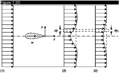Determination of profile drag with the Jones method

U,.

The third integral represents the profile drag, Dp, sum of the form (or wake) drag generated by normal stresses and of the friction drag generated by the viscous stress tensor, tm. Therefore, the profile drag, Dp, can be calculated from the equation”

«««Л (-+p-1>1 – Л ( +p 2)2 (7Л3)

Integrals of Equation (7.13) must be extended from – да to +да as for the conservation of mass is:

П(pU)i dy = J~(pU) dy (7.14)

which shows that the velocity outside the wake at the station (2) must be greater than ида in order to compensate for the flow deficit that occurs in the wake.

Taking account of Equation (7.14), Equation (7.13) can be written:

Dp = Л ( – p)y + Л P2U2 ( – U2)dy (7.15)

Since the test chamber has a finite size it is necessary to use some approximations to measure the drag profile. Of all the methods devised to calculate the drag from the balance of momentum, the most commonly used is that of Jones. This method allows the cal­culation of drag from measurements made only in the wake with an error < 2%.

In an incompressible flow, assuming that the pressure in the station (2) is equal to the pressure of the undisturbed stream, рда, i. e. that station (2) is chosen at a very large distance downstream of the airfoil and that outside the wake of the velocity U ~ ида, the integral can be extended only to the wake (from – yw to yw):

Dp =jy PU2 (U.-U )y (7.16)

Since the test chamber has a limited length, a control station (3) not far from the airfoil (e. g. after 2 – r – 3 chords) must be used. Assuming that between the stations (2) and (3) the Bernoulli theorem is valid (no turbulence in the wake):

U1 U2

P03 = Рз + PЧ3 = P – + P~2

The equation of continuity, for incompressible flow, is:

j+/’ U3dy = j+y U2dy

It is assumed that the wake has the same size in sections (2) and (3) and that the wake is not turbulent: in these two assumptions lies the inaccuracy of the method of Jones. Equation (7.16) becomes:

Taking into account Equation (7.17), the drag coefficient is calculated from:

(7.20)

To determine the drag coefficient using Equation (7.20) it is therefore sufficient to use Pitot tubes and static pressure tubes: the undisturbed stream conditions, p0x and pm, are measured upstream of the airfoil, the distributions of stagnation and static pressure in the wake section may be obtained with a wake-rake consisting of a series of static and Pitot tubes connected to a multitube manometer.

In the case of compressible flow Equations (7.17), (7.18), (7.19) and

(7.20) become:

(7.21)

1+У P3U3dy = J_7′ P2U2dy

In wind tunnels with a closed test chamber with a rectangular shape, it would be possible to calculate the lift acting on a model with a cons­tant section supported between two walls of the test chamber (two­dimensional plane flow), through integration of the pressure on the other two walls. This method stems from the principle of conservation of momentum: the lift generated by the airfoil induces an uneven distribution of pressure on the walls, which are streamlines.

Since the disturbance induced by the airfoil will propagate at infinity upstream and downstream, it should be necessary to integrate these pressures on a domain much larger than the test chamber. Therefore, a
correction factor has to be introduced to take into account the finiteness of the domain of integration.

In the case of supersonic motion, the field is necessarily limited by the intersection with the walls of the shock waves generated on the leading edge and on the trailing edge.

The distribution of the pressures acting on the model is measured in a num­ber of holes drilled normal to the surface. Measuring instruments are:

■ multitube manometer;

■ transducers each connected in succession to the holes of one or more pneumatic scanning valves (Scanivalve, see Chapter 1);

■ an electronic device scanning as many transducers as pressure taps.

Since the aerodynamic force is due to the difference between the pressure acting on the surface and the static pressure in the asymptotic stream, the tank of the multitube manometer or one of the chambers of each differential transducer is often put in communication with that pressure. The pressure coefficient

can be obtained then, in incompressible flow, dividing the readings of the differential multitube manometer by the reading of a differential pressure gage connected to a Pitot-static tube placed in the undisturbed stream.

Since the maximum pressure is the stagnation pressure, the maximum value of the pressure coefficient is Cp = 1 in an incompressible flow and slightly greater than 1 in a compressible flow. The negative pressure coefficient can reach the value Cp = -10

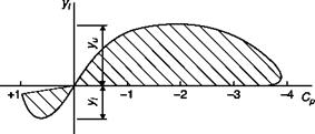
The distribution of pressure coefficients is given by a diagram in which is reported the coefficient normal to the surface (Figure 7.15) or to the main axis of the body, which, in the case of an airfoil, is the chord (Figure 7.16).

The force normal to the surface acting on an element of size 1*ds, is given by (Figure 7.15):

dF = Cpqds

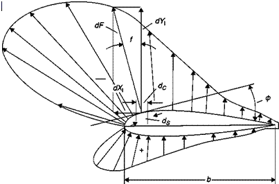From Equation (7.2) the elemental forces acting normally and along the chord can be derived

dYt = Cpqds cos ф = Cpqdc dXj = CpqdsseпФ = Cpqdy

In integrating to the whole airfoil, it must be remembered that the force acting on the lower surface must be subtracted from the force dY in each element of the chord “dc”; similarly in the calculation of the force dX on the front in each section “dy” the corresponding force acting on the back of the airfoil must be subtracted. Thus the force Y in the section is calculated by Equation (7.4) where Cp = Cpi – Cpu

Y = qJCc (7.4)

It follows that when the distribution of pressure coefficients is that normal to the chord (Figure 7.16), the distance between the upper curve and lower curve represents the distribution of loading perpendicular to the chord. The integral (7.5) represents the enclosed area:

lCfdc=A(z) (7.5)

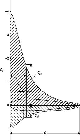Distribution of the pressure coefficients on the chord of a lifting airfoil

If the wing is not twisted, the value of Equation (7.5) can be calculated in each section and a diagram like that of Figure 7.17 can be built and the total normal force, Yt, calculated as:

Y = qZnA(zdz (7.6)

where the integral is the area of the diagram of Figure 7.17.

The total force, Xt, in the direction of the chord is calculated in a similar way by the equation:

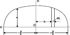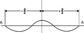
Distribution of normal force along the wing span

X = ff СрЯу = яЬ‘!ЬІ1 Z Cpdy (7.7)

where yu and yt are respectively the maximum distance of the upper and lower profile from the chord and Cp = (Cp)ant – (Cp)post.

The integral

VyCpdy = B (z) (7.8)

J yj P

is the area of the diagram Cp(y) of Figure 7.18. Bringing back to the diagram the values along the wingspan (Figure 7.19), the resultant force, Xt, can be derived from Equation (7.9) where the integral represents the area of the diagram of Figure 7.19:

X = qj h’lBd (7.9)

Distribution of pressure coefficients parallel to the chord of a lifting airfoil

Distribution of the force parallel to the chord along the wing span

Also the aerodynamic moments acting on the wing can be obtained from the distribution of pressures, for example, the pitching moment with respect to the leading edge is given by:

Mz = q[Cpxdc (7.10)

Finally, the lift, L, and the form drag, of the wing can be obtained from:

L = Yt cos a – Xtsena

Df = Ysena + Xtcosa (7.11)

It must be stressed that, lacking a measure of tangential stresses, only the part of the drag due to the integral of pressures, that is the form drag, can be obtained from pressure measurements.

Lift, pitching moment and form drag acting on a model can be determined by integrating the measured pressure distribution on the surface.

If the model is 2D (an airfoil) the so-called indirect method could also be used to calculate:

■ profile drag by measuring the losses of stagnation pressure in the wake (conservation of momentum in the direction of the asymptotic velocity);

■ lift, in a wind tunnel with a closed test chamber, by the distribution of pressures on the two walls perpendicular to those supporting the model (conservation of momentum in the direction normal to the direction of the asymptotic velocity).

The friction drag could be calculated by measuring the stagnation pressure near the surface or it could be calculated for 2D models by the difference between profile drag and form drag.

Although the determination of the forces and moments with these methods is often considered only as an alternative to a balance, it should be noted that:

■ pressure measurements provide, besides the resulting forces, a large amount of local information and, while it is possible to integrate the distribution of pressure to obtain the forces, it is not possible, conversely, to derive the distribution of pressures from the forces measured with balances;

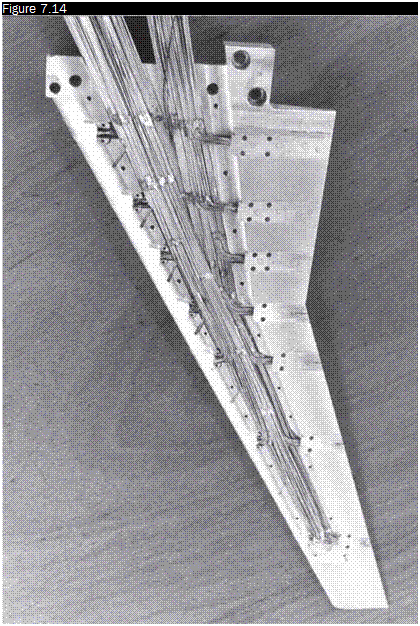
■ the determination of the forces from pressure measurements are well suited only for airfoils and 2D bodies of revolution, as in 3D models the measure of pressure becomes cumbersome even in the simplest cases and the data processing is more laborious than for measurements made with balances: an accurate 3D test requires a large number of holes and tubes, in the order of hundreds (Figure 7.14);

■ as has been said, the only possible method for the determination of aerodynamic forces on 2D models is based on pressure measurements;

■ in some cases, the model may be too small to allow a sufficient number of pressure taps to be made on the surface;

■ at supersonic speeds, the method of exploration of the wake may be inaccurate.

A wing model of a Fokker plane with 250 holes and pressure pipes

In each case, what the most appropriate method to be adopted must be evaluated. In the development of a new airplane, pressure measurements, usually combined with flow visualization, are made even when the resultant forces are measured with a balance.

Abstract: This chapter highlights methods used to measure the forces acting on a model in a wind tunnel: from pressure measurements on the surface or in the wake of the body to counterweight, strain-gage and magnetic suspension balances.

Key words: counterweight balances, magnetic balances, strain gages balances.

7.1 Types of supports for models in wind tunnels

Measuring the aerodynamic forces acting on a stationary model in a test chamber of a wind tunnel is easier than measuring the same forces on a model in free flight or put into rotation by a windmill. Nevertheless, this measure is very sensitive to the almost inevitable interference of the support system on the aerodynamics of the model that comes in addition to the interference of the walls, real or virtual, of the test chamber. Only magnetic levitation of the model is free from support interference, but so far it has been tested only on simple models in small research wind tunnels.

The support system of the model in the test chamber must allow both the necessary rigidity (it requires that the maximum error in the angle of attack be in the order of one-hundredth of a degree) and the ability to change the set-up at will (in stationary tests to evaluate the polar and in unsteady tests, with oscillating or rotating models, to measure the derivatives of stability).

Models of complete airplanes are usually supported in the center of the test chamber:

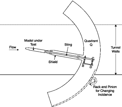
■ in the classic layout (Figure 7.1), with three parallel rigid rods (two hinged under the wings and one under the tail), the variation of the angle of attack is obtained by moving the tail support vertically; the three rods are partially shielded with fairings fixed to the floor in order to reduce their aerodynamic drag;

■ rarely used are pyramidal supports, which, as we shall see, would allow a better resolution of forces;

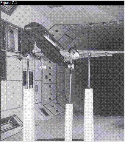Airplane model on three parallel supports in the 5-metre pressured low speed wind tunnel at DRA in Farnborough

■ in the first wind tunnels, suspension wires were used which had the advantage of not transmitting moments; with time it was found that the wakes of the threads produced more interference than shielded rigid rods and furthermore induced a drag that was ten times that of the tested model;

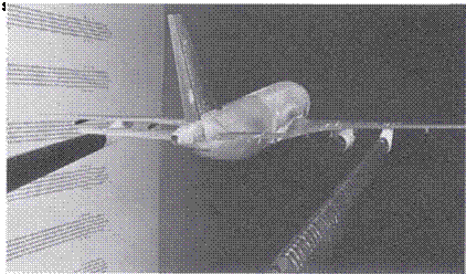
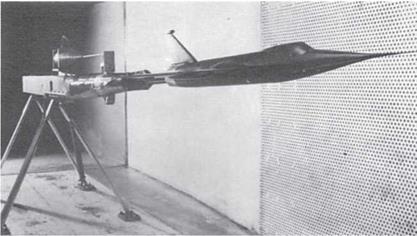
■ in the transonic field, and even more in the supersonic field, the presence of any support generates shock waves that interfere with those generated by the model. The solution consists in adopt­ing a less interfering back support (sting) that, however, since it eliminates the wake, alters the base drag. This support allows large variations of the angle of attack (Figure 7.2) and therefore is particularly suitable for testing (also in a subsonic stream) models of combat aircraft that fly with high angles of attack, even beyond stall.

The stings may take a variety of shapes depending on the model tested, the type of interference preferred, stiffness required: straight

support, double sting and Z support are shown in Figures 7.3, 7.4 and 7.5.

Airbus model on variable elbow sting in a transonic wind tunnel

If tests are performed in the presence of ground (automobiles, trains, airplanes taking off and landing, air cushion vehicles), and models are particularly heavy, the models rest on the floor of the test chamber that is also the platform of the balance (Figure 7.6), in this case the floor does not properly simulate the runway or the street since a boundary layer grows on the floor of the test chamber that is not present on the road. It is necessary in these cases that the boundary layer be removed immediately

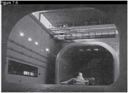
A Ferrari F-1 car in the FIAT Research Center wind tunnel at Orbassano, Turin, Italy, 1976

upstream of the model or a moving belt traveling at the same speed of the flow be provided on the floor.

A 2D model, an airfoil, must go from wall to wall in the test chamber (even in open test chambers, two parallel walls are needed to support the model), and is typically mounted on a tube going through the two walls allowing the change in the angle of attack of the model (Figure 7.7). Great attention must be paid in ensuring the seal between model and walls to prevent communication between the lower and the upper sides of the model which would lead to the formation of tip vortices, typical of finite wings, and the destruction of two-dimensionality of the motion, already compromised by the presence of the boundary layer on the two walls. In this way the model is not free to move and the aerodynamic force cannot be measured with balances and must be calculated from pressure measurements made in a row of holes on the centerline of the model.

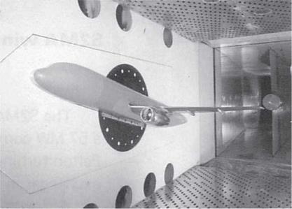
In some cases, in order to double the Reynolds number referred to the chord of the wing, half-models are used mounted on a wall of the test chamber, simulating the plane of symmetry of the airplane (ignoring in this case the presence of the boundary layer). The model is fixed on a

An airfoil NACA-0012 in the adaptive-walls wind tunnel at DIAS at University Federico II in Naples, Italy

circular support flush with the wall (Figure 7.8) with a variable incidence with respect to the direction of the asymptotic velocity.

With fixed models the behavior of the aircraft during maneuvers cannot be studied; supports oscillating in a vertical plane (Figure 7.9) or rotating (Figures 7.10 and 7.11) must be used.

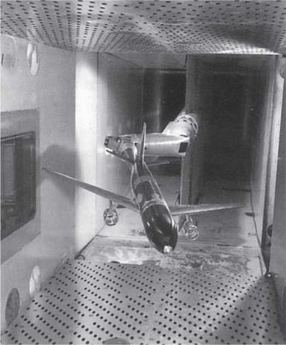
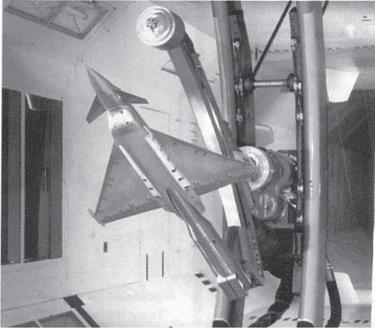
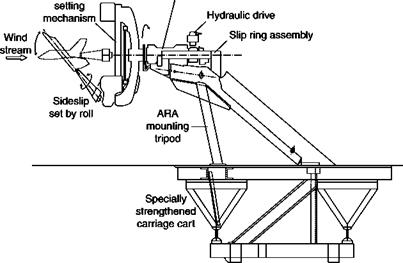
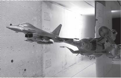
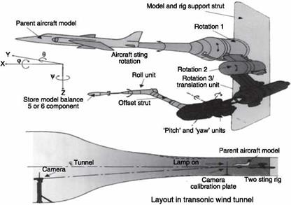
Another important problem is to evaluate the aerodynamic inter­ference between two bodies that fly close to each other: this is the case of a bomb, a missile, an ejection seat or a tank dropped from an airplane or the presence of a tanker refueling the airplane. The classic technique used to test in a wind tunnel the trajectory of loads dropped from planes is to follow with a video camera the free-fall of models of the store with a properly scaled density (models made with balsa wood), position of center of gravity and moments of inertia. At the end of the 1970s another technique was established, known as captive trajectory store testing: models of aircraft and store are supported separately (Figures 7.12 and 7.13) and the store is moved according to a trajectory calculated by a computer in real time, taking into account the inertial characteristics of the model and the measured aerodynamic forces.

A wall-mounted Airbus half-model in a transonic wind tunnel

Schematic of the rotating balance at ARA Bedford, UK

TSR (Two Sting Rig) captive store trajectory simulator at ARA, Bedford, UK

Schematic of the captive store trajectory system at ARA, Bedford, UK

Assume that the field is symmetrical about the x axis and that the direction of observation is z (Figure 6.46). The local value of the refractive index becomes a function of x and r = ^y2 + Z where r is the distance from the axis of symmetry.

Assuming that the rays of light go through the test section along the z direction, as in the case of Figure 6.46, if there is no refraction on the edge of test section, i. e. if n(rj = n0, the problem can be solved trans­forming Equations (6.10) (6.15) and (6.16) in the axially symmetric coordinate system:

In the Schlieren system:

C(y) = f y a

In the separated-beams interferometer:

In the differential interferometer:

Ml = Jr r dn(r) dr1

7 J r=y dr r-yy

The integration is performed starting from the y coordinate of the ray in question until the outer radius, rm enclosing the axisymmetric field is reached. It is assumed that the index of refraction is nm = n0 = const for r > rm, i. e. outside the test field.

Equations (6.36), (6.37) and (6.38) are integral equations of the Abel type. The quantity to be determined, n or dn/dr, must be calculated from inside the integral. In principle, there are two ways to solve this problem. The first way is analytic (Abel inversion). The solution can be obtained by applying to both sides once again the operator

d(y)

l~2 2

Vr – y

and reversing the order of integration in the double integral created at the second member. For example, in the case of separated-beams inter­ferometer, Equation (6.37), the Abel inversion provides:

The integration should be done on the measured function Ml (y), difference of the optical paths. Since this is available as a set of discrete values, these values should be fitted with an appropriate analytic function. A disadvantage of this approach is the further differentiation of the function needed in Equation (6.39).

Applying the Abel inversion to Equations (6.36) and (6.38), is obtained directly:

In the first member of Equation (6.38), the approximation was made:

Surprisingly the results for the differential interferometer, Equation (6.41), and the Schlieren system, Equation (6.40), are less complicated than that for the separated-beams interferometer, Equation (6.39), because the index of refraction can be achieved without the need for additional differentiation of the function approximating the experimental data.

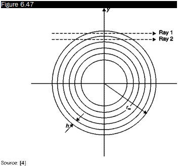Subdivision of the axially symmetric field in annular zones with thickness h

The second method for solving the axially-symmetric problem prevents the use of the Abel inversion through a numerical procedure. To this end, the cross-section of the axially-symmetric field is divided in rings of radius r (Figure 6.47). The amount to be determined is a supposed constant in each zone. The procedure is a step-by-step solution that starts from the outer edge rM of the field and can be easily computed.