Category Aerodynamic measurements

6.8.1 Problem set-up

The objective of the analysis is the determination of the function n(x, y, z) by Equations (6.10), (6.15) and (6.16) depending on the type of optical system: Schlieren, separated beams interferometer or differential interferometer, respectively. In general, this problem has no solution, unless the test field shows some kind of geometric symmetry allowing a reduction of the independent variables of the function n(x, y,z) from three to two.

The analysis of an arbitrary field would require many images of the field taken from various angles. If the field has some symmetry, the num­ber of images required is reduced: a single image is sufficient in the case of a two-dimensional plane field or of an axially symmetric field with an axis of symmetry normal to the direction of observation.

6.8.2 2D plane fields

Equations (6.10), (6.15) and (6.16) can be immediately solved if the index of refraction n is independent of z, i. e. if n = n(x, y). Quasi two­dimensional fields can be achieved in a test chamber of a wind tunnel if the model has a constant section and extends from one window to the other, and the direction of the rays, z, is normal to the entry windows. The presence of the windows is equivalent to a jump in the index of refraction along the z axis.

In the case of a Schlieren system, light rays pass undisturbed through the first window of the test chamber, which is normal to the direction of the rays, all parallel to the axis z (Figure 6.45). On the output window, a ray deflected of the angle 6x, given by Equation (6.7), will pass in the outside environment, of refractive index na, with the angle given by the equation:

nsen°a= nsenex ^ da = ne* (6.27)

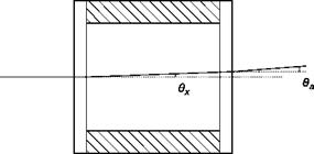Deflections of light rays passing through a test chamber bounded by two glass windows

Then the local contrast, for Equations (6.10) and (6.27), is given by:

) DI(x, y) fL 1 dn(x, y)

Cx, y) = – = a I a na dx

The index of refraction can be calculated in a point (x, y) by integrating the measured contrast on a Schlieren image from a point (x0, y), where the index is known, through the equation:

n(x, y)- n(x0,y) = XC(x, y)dx (6.29)

f L x0

In the case of a separated-beams interferometer, the effect of the windows is eliminated by including in the reference path two compensation plates having the same thickness and the same quality of the windows, or by passing the reference beam in a zone of the test chamber where density is a constant. Equation (6.15) gives then:

і D (x, y) • / D (x, y) ІҐ in

n(x, y)-n0 =——— L—— 1-e- P(x, y)-Po = K(X)L (6-30)

In the case of differential interferometry, the effect of the windows of the test chamber is irrelevant because both interfering rays pass through the test chamber and then through the same windows. The index of refraction can be calculated by Equation (6.16):

(6.31)

In both classes of interferometers the difference of optical paths can be related to the displacement of the fringes, Aw, and to the wavelength, l, of light. The displacement of the fringes produced by the disturbance is given by:

The sensitivity, s, of the interferometer is defined as the fringe shift divided by the jump of index of refraction

Aw(x, y)/w A (x, y) L

An(x, y) XAn(x, y) X

Equations (6.30) and (6.31) allow, taking into account Equation (6.32), the calculation of the index of refraction in terms of fringe shift:

p ( x ) x

n(x, y) — n0 + b ^ ^ — separated-beams interferometer (6.30′)

X x

n(x, y) = n(x0,y) + ^-^J p(x, y)dx differential interferometer

(6.31′)

In the case of infinite width fringes, the resulting fringes are curves of constant refractive index (separated-beams interferometer) or curves of constant gradient of refractive index (differential inter­ferometer). Recalling Equation (6.13), the difference in refractive index between two consecutive fringes in separated-beams interferometer is simply:

(6.34)

and the difference in gradient of refractive index between two consecutive fringes in the differential interferometer is:

/^ЭлЗ X

UxJw+1 UxJw Ld

The simplest differential interferometer [10] consists of a glass plate on which the rays reflected from the first and the second surface of the plate are made to interfere. The plate can be put immediately after the test chamber before the second mirror of the Schlieren system. In this case, a beam of parallel rays hits the plate (Figure 6.41): ray 1 is reflected in part on the upper surface of the plate (ray 1′) and partly propagates within it undergoing a refraction in passing from air to glass. The ray refracted, in turn, partly passes into the air and is in part reflected by the lower surface and refracted through the upper surface (ray 1"). Among all the rays that reach the plate, there is a ray 2 that produces a reflected

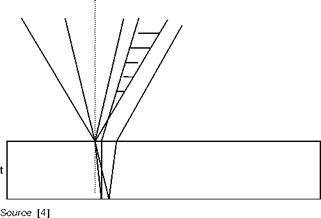
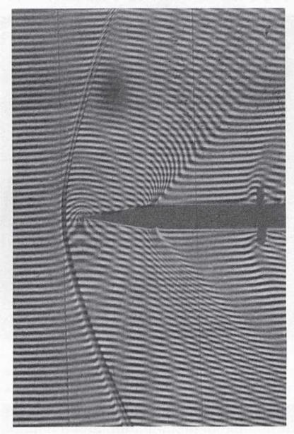
Schlieren interferogram of a shock wave with vertical or oblique fringes

Exact position ^ of shock wave

ray 2′, overlapping 1" and giving rise to interference. Similarly, there is a radius 3 that generates a ray 3′ interfering with the ray 2", and so on. The difference in optical path between interfering rays is equal for all rays and is given by the geometric path of the refracted ray in the slab, multiplied

Figure 6.41

by the refractive index of glass, nv, minus the path in air of the ray reflected from the upper surface, multiplied by the refractive index of air, na.

With simple geometrical considerations it is easy to write

M = 2tt]n2r – n2a sin2 i (6.23)

where t is the thickness of the slab and i is the angle of incidence of the beam on the plate.

If the beam has passed through an object with a constant density, inter­ference fringes are not formed and the uniform brightness of the beam downstream of the plate (no fringes) depends on the optical path diff­erence given by Equation (6.23). If the density of the test field is variable, interference fringes are formed that are loci of equal density gradient.

Separation distance between the interfering rays is given by

tna sin2i

2 • 2 •

nv – na sin i

In fact, in this type of interferometer, rays that interfere are more than two because there are multiple reflections inside the slab, for example, there will be a radius 1’" which also interferes with the radius 3′, but successive reflections decrease in intensity and thus contribute more and more negligibly to the phenomenon of interference. Apart from the inability to generate finite width fringes, this type of interferometer is limited due to the fact that a plate of interferometric quality, which is therefore expensive, is needed.

These constraints can be removed if the plate is in the focus of the Schlieren system replacing the knife edge. The cone of light reflected from the first face of the plate interferes with the one refracted and then reflected from the second surface of the plate (Figure 6.42). The area of the plate affected by the cone of light is the order of mm2 and therefore the quality of the slab is virtually irrelevant.

Since the single rays have different incidence on the plate, the optical paths are different from ray to ray, so even in the case of a uniform field, fringes will be present (finite width fringes), the width of which is at a first approximation inversely proportional to the thickness of the slab. The distance of separation of the rays that interfere at a distance D from the focus is given by:

Reflection plate interferometer in the focus of a Schlieren system

Separation varies with the angle of incidence and therefore the sensitivity varies from point to point in the test section. The thickness of the fringes is given approximately by:

The choice of the angle of incidence is dictated by the need to have fringes as far as possible straight, parallel and of uniform thickness. Since the reflected rays from the first and second face of the slab can be considered as coming from two point sources, the surfaces of interference, constructive or destructive, are hyperboloids of revolution (Young’s experience) that are the loci of points which have a constant geometric path difference between the two coherent sources in phase with each other (Figure 6.43).

It is obvious that the shape of the fringes depends on the position of the observer with respect to the line joining the two light sources (axis of revolution of the hyperboloid): circular, elliptic or hyperbolic fringes can be observed with increasing angles between the direction of observation and the axis of revolution.

In Figure 6.44 are shown fringes obtained at different angles of incidence with three plates of different thickness. With all the plates fairly straight and parallel, fringes are obtained with angles around 45°. At small angles of incidence, fringes are curved; at too large angles of incidence, the phenomenon of multiple reflections will take place with a

Standing waves produced by two sources in phase; on right, equal phase surfaces (hyperboloids)

loss of sharpness of the fringes. Few fringes are generated by the thinner slide (t = 0.15 mm) and fringes too numerous and almost indistinguishable with the thickest one (t = 1.60 mm).

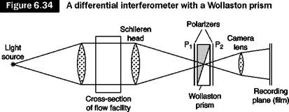
A scheme of this type of differential interferometer is shown in Figure 6.34. The configuration is similar to that of a Schlieren system in which the knife is replaced by a Wollaston prism between two crossed polarizers. In its no-fringe basic configuration, the center of the prism coincides with the focus of the second Schlieren lens [9].

The Wollaston prism (Figure 6.35) consists of two prisms of bi-refracting material such as quartz or calcite, glued together so that the optical axes of the two prisms are mutually perpendicular. The effect of the prism is to separate a ray of incident light into two diverging rays that are linearly polarized in directions perpendicular to each other.

An incident ray is in fact separated in the first part of the prism in an ordinary and an extraordinary ray that propagate at different speeds and are therefore subject to different indices of refraction, no and ne. Due to the orientation of optical axis, the ordinary ray of the first part of the prism becomes extraordinary for the second prism and vice versa, so these two components are separated by an angle b = 2a(ne – no), considering that the angle a of the prism is small.

The incident ray 1 is thus separated into two rays 1′ and 1° polarized and forming an angle b (the symbols ‘ and ° indicate the direction of polarization in the plane of the figure and perpendicular to it respectively). In the convergent beam, hitting the prism is ray 2 forming an angle b with ray 1, which is separated into 2′ and 2°; ray 2’ therefore overlaps 1° and they may interfere only if they have an equal polarization direction; this condition is achieved through the polarizer, P2 which is rotated 45° with respect to the two directions ° and ‘. The optical axis of the polarizer P1 is parallel or normal to that of the polarizer P2 in order to make the two interfering beams of the same intensity. The same procedure applies to rays 1 and 3 (1’ and 3° can interfere), and so on. The interfering rays come from different points of the test chamber, which they crossed separated by a distance d = b*f2. If these rays pass through regions of different refractive index, they have a phase difference that produces interference.

The edges of rigid bodies normal to the separation distance d will appear with a double image or gray zone of thickness d (or d*cosy where Y is the angle between the normal to the edge and the separation dis­tance d). The formation of this double image is due to the fact that the wall stops one of the two beams that should interfere.

A shift s of the prism along the optical axis of the lens with respect to the focus of the Schlieren involves the formation of parallel and equidistant fringes on the screen. The thickness of the fringes in this mode of operation, fringes of finite width, is inversely proportional to s:

w = Ts = d (6.22)

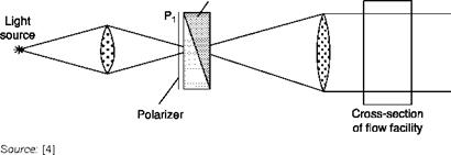
A rotation of the prism around the optical axis causes the rotation of the system of fringes. The configuration shown in Figure 6.34 requires a point light source or a laser. If such a source is not available, a configuration with two Wollaston prisms has to be used: the rays of light separated in the first prism are recombined in the second prism (Figure 6.36). The purpose of the first prism is to improve optical coherence and it is clear that the two prisms must be identical.

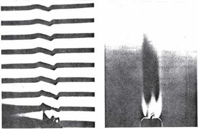
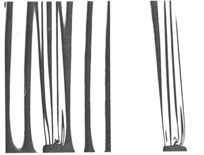
Figures 6.37, 6.38 and 6.39 show the interferograms of a candle flame obtained with oblique, horizontal and vertical fringes and with zero fringes.

Of particular interest is the visualization of a shock wave. Due to the high density gradient across the wave, the configuration of the fringes cannot be treated with the linearized Equation (6.16) and the full Equation (6.14) must be taken into account. Only the pairs of conjugate rays that pass one upstream and one downstream of the shock wave can contribute to the formation of the configuration. The wave, with infini­tesimal thickness, appears thick d or dcos/in analogy with the formation of double image of the edges of rigid bodies already described above.

In the method of pre-existing fringes, the shock wave cannot be

Interferometer with two Wollaston prisms; shown here is the light source side, the right side is equal to that of Figure 6.34 without the polarizer P±

Schlieren interferogram of a candle flame. Oblique fringes; on right, zero fringes

Schlieren interferogram of a candle flame. Horizontal fringes; on right, zero fringes

Schlieren interferogram of a candle flame. Vertical fringes; on right, zero fringes

displayed with fringes normal to the wave (y)= 90°). It is not convenient to have fringes parallel to the wave, it is preferable to use oblique fringes (Figure 6.40); from the relative displacement of the fringes it is possible to calculate the density jump across the wave.

In the preceding paragraph the assumptions of monochromatic and point light source were made. The basic requirement, in order to ensure that the two intersecting beams give interference, is that the phase difference of rays remains constant in all the observation time. This is linked to conditions on the spectral amplitude of the light emitted (temporal coherence) and the finite extension of the source (spatial coherence).

Consider the extreme case of only two sources whose wavelengths differ by D1: the system of fringes disappears when the Nth bright fringe produced by the light with wavelength 1 falls on a dark fringe produced by the wavelength 1 + D1. The difference in amplitude of the fringes is, for Equation (6.19) Dw = D1/2e and the condition of cancellation of the fringes is:

,,, w Л7 Я

NDw = — ^ N =————-

2 2АЛ

then with a given 1 and a given amplitude of the spectrum of the source, the equation allows calculation of the maximum number of fringes that can be obtained: for red light (1 = 632.8 nm) and an interferometric filter with bandwidth, D1 = 1 nm, about 300 fringes can be generated.

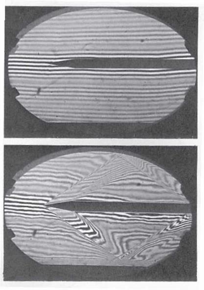
With a white light fringe, this phenomenon clears all except the white fringe of zero order and a few colored fringes on each side of it (Figure 6.32, top). This particular feature is used to follow the fringe shift through a shock wave: with the white light it is very easy to follow the brightest zero-order fringe (Figure 6.32, bottom).

A finite source may be regarded as consisting of many source points, so in every point on the screen the light intensity is the result of some interfering pairs rather than a single pair. The interference is obtained only if the difference in optical path between a pair of ray changes by no more than 1/2 on the whole source.

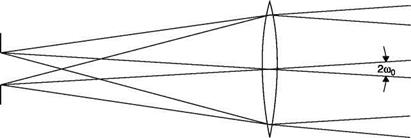
From Figure 6.33, we can see that there are a number of beams of parallel rays from each point of the source entering the interferometer; between the two extremes there is an angle of 2w0. If the central beam enters the interferometer at 45° from the surface of the first beam-splitter and if the produced fringes are perpendicular to the plane of the centers, from simple geometric considerations it can be found that the maximum number of fringes in the field is:

(6.21)

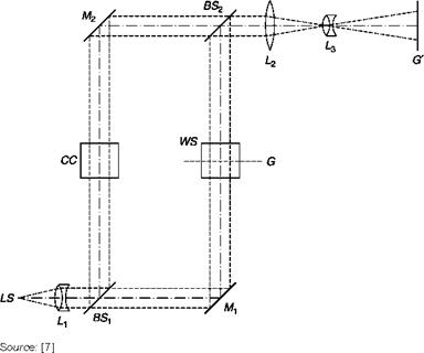
It is also difficult to obtain good contrast of the fringes in the presence of dispersion in the various optical components. The limited spatial and temporal coherence of the normal light source, usually mercury arc lamps filtered with a narrow band interferometric filter (AX = 1 nm), implies the need for strictly equal path lengths which limits the tolerance in the initial assessment of the instrument to a few wavelengths. If the test chamber has windows, these introduce an optical path difference between the test and reference beams of the order of a few centimeters and it is therefore necessary to make the two path lengths equal, introducing into the reference path a pair of glasses identical to the windows of the test chamber (the compensation chamber, CC, of Figure 6.27) or by passing also the reference beam through the test chamber in an area where the density is constant and is known.

In practice, the Mach-Zehnder interferometer requires five adjustments and high quality precision optics: all optical surfaces, including the windows in the test chamber, must be machined with great precision, so that the thickness of the mirrors must be constant within a tolerance of less than X/12. This type of interferometer requires adequate structural rigidity and must operate in the absence of vibrations that could alter the optical path difference between the two beams.

Using a gas laser, which acts as an ideal point source for monochromatic and coherent light, the coherence length is of a few decimeters (see Chapter 4) and most of these difficulties disappear. The use of a laser has the following effects:

■ tolerance in the initial set-up of the interferometer is of some decimeters;

■ there is no need to make equal the thickness of the optical components

in the two paths;

■ a large number of well-contrasted fringes is easily obtained;

■ three of the five fine adjustments of the interferometer become

redundant, there remain only the controls on spacing and inclination of the fringes.

Unfortunately, the coherence of laser light introduces new difficulties:

■ the rear surface of the beam splitters and each surface of the windows of the test section reflect light in the direction of the main beams: since this light is coherent with that of the main beams, spurious fringes are generated that may also have a high contrast; this phenomenon can be eliminated by treating the concerned areas with an anti-reflective coating (e. g. MgFl2 reflecting only 4% of incident light);

■ laser light is diffracted on each object placed in the beam out of focus, including dust particles and fingerprints on lenses and mirrors: diffracted light is coherent and produces other spurious fringes; this requires an extreme and continuous cleaning of the optics surfaces. The problem is greatly alleviated if the laser beam is passed through a spatial filter (see Section 4.2.5).

The main advantage of this type of interferometer is the fact that the two path lengths can be separated at will so that tests can be made also on very large objects, such as test chambers of wind tunnels.

The beam of parallel rays coming from the light source LS (Figure 6.27) is split into two beams by a beam splitter, BS1, covered with TiO2, which reflects approximately 35% of incident light, placed at 45° with respect to the optical axis. After reflection on the two mirrors, Mx and M2, covered with aluminum that reflects at least 90% of incident light, the two beams are recombined downstream of the beam splitter BS2. The working section, WS, is located between Mt and BS2 in Figure 6.27, but it could be located in any one of the sides of the rectangle at will.

Since the interference fringes are generated downstream of the beam splitter BS2, there is a problem of focusing contemporarily two objects (the fringes and the test section) at different distances from the screen G’: in order to do that, the lens L2 is inserted downstream of BS2 in order to produce a virtual image of the fringes at the center of the test chamber. To enable fine-tuning of the focus, the beam splitter, BS2, has a translational degree of freedom.

If the four plates are exactly parallel to each other, undisturbed waves arrive in BS2 perfectly in phase with each other so that the light intens­ity on the screen is uniform. The method is called infinite width fringe or zero fringes.

If a change in density is introduced in the test chamber, the phase change that develops produces interference fringes which are lines of constant density (Figure 6.28). The difference in optical path between two consecutive fringes is equal in absolute value to a wavelength.

The number of fringes that are generated, and therefore the resolution that can be achieved in identifying the density distribution in the field, depend on the variations of density and therefore cannot be controlled by the operator.

If a better resolution is needed, straight and parallel fringes can be generated: this may be achieved by rotating of a small angle, e, the beam splitter BS2 around an axis normal to the plane of Figure 6.29. A purely geometrical optical path difference between the pair of conjugate rays that meet at P is thus generated given by:

At = OP-OC = 2b —1 — ) = 2btane = 2be (6.17)

V sen2e tan2ej

which is the same for all points on the normal to the plane at P, so straight fringes are produced parallel to the axis of rotation of the beam splitter, as shown in Chapter 4 for the crossed-beams laser-Doppler anemometer.

Contour interference fringes obtained with the zero fringes method

At point O and, provided that the angle 2e is small enough, all along its bisector rays with the same optical path interference and then at the point O’, there is the fringe of order 0. Assuming that N bright fringes exist between O’ and P, the difference of optical path length for the rays meeting in P is:

M = NA = 2be

Therefore, the distance between two consecutive fringes is given, in agreement with Equation (4.8) for small angles, by:

The introduction of a disturbance in one of the two optical paths produces a fringe shift (Figure 6.30). If a fringe moves one fringe thickness compared to the corresponding position in the undisturbed stream, this

means that the difference in optical path is changed by one wavelength, in absolute value. With a simple measurement of displacements as multiples or submultiples of fringes width, the density variations can then be calculated with the desired resolution.

Contour fringes can be obtained also with the system of finite width fringes by superimposing a no-flow image on an image obtained in the presence of flow. The regions where the fringes are displaced of Nl become visible as bright stripes that represent points of equal density, or isopicnals (Figure 6.31).

Two beams interferometry is based on the comparison between the optical paths of pairs of light rays that pass through a test field in which the index of refraction, n, is not homogenous. The optical path traversed by a light ray is defined as the curvilinear integral

I = J n(x, y,z)ds (6.11)

where ds is an element along the path and n(x, y, z) is the distribution of the index of refraction in the test field. (In a vacuum, where n = 1, the optical path coincides with the geometrical path.) Pairs of coherent light rays that travel different optical paths can create interference, in particular, negative interference, a black point, if the difference between the optical path of the two rays is equal to an odd number of half wavelengths, see Equation (4.7):

M = ± (2^+ 1)j [n = 0, 1, 2……… ] (6.12)

and positive interference in a point, where the brightness is equal to four times the brightness of the single rays, see Equation (4.7), if the optical path difference is equal to an even number of half wavelengths (a multiple of wavelengths):

M = +2N— = ±N—

2

In the image of the test chamber, a pattern of stripes, interference fringes, is generated. This phenomenon occurs only if the two interfering beams are generated by coherent sources (i. e. sources that emit light waves with the same wavelength and constant phase difference). Because it is impossible to obtain two distinct and perfectly coherent sources, it is necessary to use a single source and split the beam into two beams which are then recombined.

In order to introduce a classification of different systems it can be assumed that all light rays are straight and parallel to the axis z. Assume that the pairs of conjugate rays lie in the plane x, z (Figure 6.26) and that in the test field are separated by the distance d. If the coordinates of the two input rays in the test field are indicated by Z and Z2, and the coordinates of output with Z and Z2, the difference in optical pathlengths of the two rays is given by:

(6.14)

Unfortunately from this equation it is not possible to determine n(x, y, z) since in it are two unknowns: the distribution of the refractive index

Figure 6.26

along two trajectories. All systems used for optical interferometry reduce the number of these unknowns to one. One can identify two types of different devices depending on the distance between the two rays and therefore interferometers will be classified as separate beams inter­ferometers and differentials interferometers.

If D is the diameter of the test field, when d/D > 1, one of the two conjugate rays will pass outside the test field, usually through a medium with a constant and known refractive index n = n0 . These rays form a reference beam that is made to interfere with the test beam. The difference in optical path in this case is:

where L is the size of the test chamber in the z direction. The separate beams interferometers are therefore sensitive to the absolute change in refractive index or density. The typical instrument of this class is the Mach-Zehnder interferometer.

Differential interferometers are characterized by a very small ratio between the separation of the rays and the diameter of the test field, d/D << 1: in practice, both the two conjugate rays pass through the test field, separated by an infinitesimal distance d. These interferometers are also called Schlieren interferometers because the optical apparatus is very similar to the Schlieren system.

Developing Equation (6.14) in a Taylor series truncated at the linear terms, since d is infinitesimal, we have:

similar to Equation (6.10) for n = 1.

Many differential interferometers have been made, some of them can only operate using a laser as a light source, the most commonly used is the Wollaston prism interferometer.

There are many advantages using differential interferometers with respect to separated beam interferometers:

■ separated beams interferometers cannot be used whenever the difference in optical paths between the two beams is higher than the coherence length (the presence of thick glass windows in one of two paths);

■ in a differential interferometer, since both the interfering rays pass in the test chamber separated by an infinitesimal distance, they are equally affected by any vibration;

■ differential interferometers do not require the elaborate and sophisticated alignment procedures needed in separated beams interferometers;

■ differential interferometers can be made in large dimensions because the mirrors used, which are the same of the Schlieren system, easily reach a diameter of 50 cm, with costs much lower than those of the high quality optical components of a Mach-Zehnder inter­ferometer;

■ the cost of a differential interferometer is extremely low because the optical components of the Schlieren equipment are usually already available in any fluid dynamics laboratory.

Any apparatus that produces images in which the brightness depends on the local deviations that light rays undergo when crossing the test zone is generally classified as Schlieren. Strictly speaking, the shadowgraph is also a Schlieren, but currently this name is attributed solely to the method proposed by Toepler in 1866.

In this system (Figure 6.20), a first lens produces a beam of parallel light rays passing through the test chamber, a second lens produces an image of the test chamber on a screen and an image of the light source in its focal plane. A knife edge or cut-off is introduced into the focus, to cut a fraction of the image of the source.

To understand how the system works, it should be noted that the light source is of finite size, usually rectangular 10 mm x 1 mm (Figure 6.21,

bottom left). Each point of the source (Figure 6.21) produces a pencil of parallel rays passing through the entire test chamber and is focused in a point; the focus consists of the focal points of all the pencils that have crossed the test chamber, bearing with them all the information. In the absence of disturbances in the test chamber, cutting part of the focus with a knife edge only makes the light on the screen reduced, without any loss of part of the image of the test chamber on the screen. The loss in brightness is proportional to the fraction of the image of the light source cut by the knife edge, (b – a)/b, where b is the height of the light source and a is the height of the part of it not intercepted by the knife edge (Figure 6.22b). Usually the knife cuts half of the focus (a = b/2).

On the other hand, every ray that passes through the test chamber is the sum of rays coming from all the points of the source and focuses on all the points of the image of the source, and for this reason the image of

Pencil of rays generated from various points of a light source of finite size. In detail at the bottom left the system used to generate a rectangular source

Source: [5]

the source can be thought of as the overlapping of all the images produced by all the rays passing through the test chamber.

If there is a density gradient in the test chamber, the ray passing through that point is deflected either upwards or downwards depending on the sign of the density gradient, and the corresponding image of the source moves by ±Da with respect to the knife edge and then is cut more or less than other images of the source formed by the undisturbed rays (Figure 6.22b). This shift and the resulting change of lighting of the corresponding point on the screen are proportional to the deflection angle.

Assuming that Qx is small, from Figure 6.22a is obtained that:

Da(x, y) = /2tan0x(x, y) = fAU, y) (6.9)

When Da(x, y)/a = ±1, the maximum deviation angles, Qxmax, is reached, beyond which no further changes occur in brightness (saturation o/ Schlieren) because the source images are either completely cut by the knife or not cut at all.

The contrast at the point (x, y) of the image is given, for Equation (6.6) and Equation (6.9), by

Al(x, y) Aa(x, y)

a

dlnn(x, y)dz_ вх (x, y) dx #

The sensitivity, s, defined as the relative deflection, Aa(x, y)/a, obtained at the knife for the unit deflection of the ray in the test chamber

a 0X (x, y) ex

increases with the focal distance of the second lens. To increase the sensitivity, the value of b = 2a can also be reduced, but this means a decrease in global brightness. An excessive sensitivity may otherwise not be desirable because even the small gradients of density present in the laboratory are magnified, thereby introducing a noise in the image.

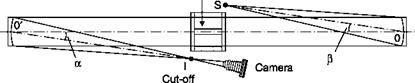
Note that the Schlieren system is only sensible to the component Aa(x, y) of the displacement normal to the knife edge (Figure 6.22b); since this shift is a function of the gradient of the refractive index in this direction, the knife must be oriented appropriately depending on the phenomenon to be visualized (normal shock wave, oblique shock wave, boundary layer, etc.). Although a rectangular source and a straight-edged knife are commonly used, rarely for particular applications can other shapes be used, for example, a circular source and a ring knife can be used if a uniform sensitivity in all directions is required. Usually on the photos obtained with the Schlieren system are reported the type and orientation of the used knife edge to make easier the interpretation of the image (Figure 6.23).

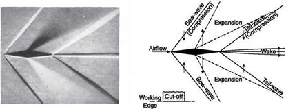
In Figure 6.24, the Schlieren images for different operating conditions of a de Laval nozzle are shown.

Since the eye is more sensitive to changes in color than in brightness, it is preferable to use Schlieren configurations that obtain color images in which every nuance of color corresponds to a particular density gradient in the flow. One approach is easily achievable replacing the knife with some transparent and colored parallel stripes, made of sheets of cellulose acetate or gelatin filters. No more than three colors are generally used and the three-color filter is positioned parallel to the light slit. The combination red-yellow-blue gives the better contrast: the undisturbed

Schlieren photograph of a double wedge in a flow at M = 1.6 and its interpretation

field is yellow, the gradients deflecting the rays in a direction give red zones and those deviating them in the opposite direction give blue zones.

Using Equation (6.10) quantitative results from a Schlieren could be obtained using a photodensitometer on the photographic negative. Quantitative results could also be obtained by doing a direct scan of the focal plane of the Schlieren system with a photomultiplier. In practice, significant difficulties arise in the accurate photometric analysis of the image, and also for the aforementioned problem of saturation: this can be avoided only if the knife is replaced by a gradual filter with various shades of gray. Once again, the filter should be placed so that the direction of change of gray is in the same direction of the density gradient to be measured.

The Schlieren system is usually not used to get the value of density, but is extremely useful in the qualitative description of the test field.

For the large diameters (D > 100 mm) required to illuminate the win­dows of a supersonic wind tunnel, lenses are usually replaced with concave mirrors; in fact, a mirror is easier to build and less expensive than a lens because:

■ the internal quality of the glass is not important;

■ it is necessary to work on only one surface;

■ a mirror absorbs less light than a lens;

■ chromatic aberration is eliminated.

Mirrors with a protecting glass, like those for home use, cannot be used since a double reflection is produced, the first on the covering glass and the second on the mirror surface. The reflecting surface must therefore be exposed to the air: aluminum is usually used, because its oxide (Al2O3) is transparent.

Schlieren images of flow in a supersonic nozzle at different ambient pressures

When using mirrors, the source and the knife should be placed outside the optical axis (Figure 6.25) the mirrors should be in the form of an offset paraboloid. The production of mirrors of this type, however, is

Z-configuration of a Schlieren system with mirrors

expensive and spherical mirrors are preferred; this approximation is allowed if the ratio between focal length and diameter of the mirror is more than 10.

To minimize the aberrations due to a spherical mirror, the offset angles a and b of Figure 6.25 must be small and also of opposite sign so that the source and the knife are on opposite sides of the axis of the two mirrors. The first precaution minimizes the effects of astigmatism, the second, the effects of coma. It is also necessary that the astigmatism distorts the image only in the direction parallel to the edge of the knife; this may be done by placing the source, the knife and the optical axis of the system in the same plane.

If the flow field is traversed by a light beam (Figure 6.16a), the image that is formed spontaneously on a screen perpendicular to the axis of propagation is called a shadowgraph. If the beam is made parallel by a lens (Figure 6.16b), the shadow will have the same aspect ratio as the model. The images produced are carriers of information so implicit that it is very difficult, if not impossible, to infer density variations from an examination of the image.

The shadowgraph method: (a) divergent light rays; (b) parallel rays

To understand the operating principle of the shadowgraph in detail, the behavior of the index of refraction within the field must be considered. Let AB and CD (Figure 6.17) be the undisturbed paths of two adjacent rays. If there is a variation in the index of refraction, the rays are deflected: if the gradient of the index of refraction, Эл/dx, is constant, i. e. Э2 л/ dx2 = 0, the two rays are deflected by the same angle and remain parallel (Figure 6.17a): the illumination on a screen placed down­stream of the test chamber is uniform. If d2nf dx2 > 0, the deflected rays diverge (Figure 6.17b), because the ray passing in A meets zones with a stronger gradient of index of refraction with respect to the gradient met by the ray passing in C; a darker zone is generated on the screen. Finally, if d2n/dx2 < 0, the rays converge (Figure 6.17c) and a brighter zone is obtained on the screen.

The shadowgraph is successfully used for the visualization of surfaces of discontinuity in the index of refraction (density) like the shock wave, or of layers with strong and variable density gradients (dynamic and thermal boundary layers).

Effects of the gradient of refractive index on the deflection of light rays

Evolution of density, its gradient and the gradient of gradient within a shock wave

Consider, for example, the case of a jump in density across a shock wave (Figure 6.18). In the same figure are shown the evolution of density and of the gradient of the gradient of density inside the wave, con­sidered of finite thickness. In the front of the wave Э2л/dx2 > 0and the screen displays a dark line, in the back д2п/dx2 < 0and the screen displays a bright line. Therefore a shock wave appears on the screen as a succession of two light bands: the first dark and the second bright (Figure 6.19).

Shadowgraph of shock waves and wake on a sphere in a stream at M = 1.6

It can be shown that the contrast of light, C, produced at each point of the screen is given approximately by:

where I is the light intensity and £ is the distance of the disturbance from the screen.

Calculation of density from Equation (6.8) requires a double integration of the local contrast (appropriate devices are needed to measure the light intensity). Moreover, Equation (6.8) becomes less reliable in the description of phenomena that are best viewed with the shadowgraph (i. e. discontinuities in the value of the index of refraction). In fact, large variations in the density gradient will produce, starting from a certain distance from the phenomenon, an intersection of the various rays that destroy the correspondence between points of the test field and the image obtained on the screen that is the basis of Equation (6.8).

The shadowgraph is very simple from the viewpoint of the optical components required, and is useful for the visualization of fluids in which there are discontinuities in density, but it is essentially a qualitative method as the calculation of the distribution of the index of refraction from Equation (6.8) seems rather difficult, if not impossible. One can say briefly that with this method small changes in n are not detected and large variations in n cannot be calculated.

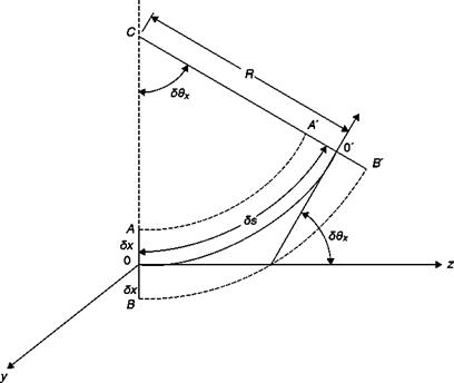
Assume that the beam, which initially propagates in the z direction, encounters a zone where there is a gradient of refractive index

Deviation of a light beam in the presence of a constant gradient of refractive index

(Figure 6.15). Denoting with n the refractive index at the point 0, at points A and B of the beam, at a distance of ±8x from the z axis, the refractive index takes the values respectively:

Эл Эл. ,

nA = n+——ox nB = n – — ox (6.3)

dx dx

Since there is an inverse relationship between the refractive index and the speed of light, c, the speed of light at points A and B is such that:

dn s

л——- ox

dx dn „

n+— ox dx

therefore, the beam deflects toward the positive x axis. After a time, 8t the wave front AB is in the position A’B’ deflected by the angle 8Qx with

respect to AB. The rays passing through A and B in time 8t travel distances SsA and 8sB proportional to the speeds cA and cB, respectively. Indicating with R the radius of curvature of the ray passing through the origin of the axes, we can write:

which yields:

which is the required relationship between the deflection of the light rays and the gradient of the index of refraction.

Similarly, if there is a gradient of n in the y direction, constant and greater than zero, the beam undergoes a deflection towards the positive y axis given by:

So, =1 ^Ss

n dy

The total deflections that the beam suffers through a test chamber of width L are therefore, respectively:

where s can be replaced with z as the deviations are usually infinitesimal.

Optical methods allow the detection of density variations that occur in a fluid due to changes in temperature and/or speed and/or composition. The principle on which these methods are based is that the variation of density, p, produces a variation of the refractive index, n, of the fluid which in turn influences the trajectory (refraction) and the phase of the light rays that pass through the fluid. Appropriate optical devices convert the resulting effect in changes of light intensity on a screen or on a photograph.

The index of refraction, n, of a transparent medium, which is the ratio between the speed of light in vacuum and the speed of light in the substance, is related to the density by the Lorenz-Lorentz equation:

where R (l) is, for each substance, a function of the wavelength, l of the light.

When the index of refraction n = 1, as in the case of gases (see Table 6.1), Equation (6.1) can be expanded in series and, stopping the

series at the first two terms, the simpler Gladstone-Dale equation is obtained:

n = 1 + K(X) p = 1 + ^( ) p (6.2)

Ps

where K(l) = 1.5 R(l) and ps is the density at standard conditions (T = 0°C, p = 760 mmHg).

The values of P for some gases are reported in Table 6.2.

Changes in the Gladstone-Dale constant with the wavelength are limited to a few percentages (see Table 6.3).

Effects of a change of refractive index on a light ray

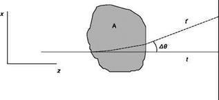
Assume that the fluid is confined in a region of space and that the region is crossed by a beam of parallel rays of monochromatic light that propagate along the axis z. A generic ray (Figure 6.14), in the absence of disturbance, i. e. the properties of the fluid are uniform in the region, reaches the screen at the point P at time t; if the fluid properties are not uniform, the trajectory of the ray deviates of an angle A© from the straight line due to the phenomenon of refraction and the ray reaches the screen at the point P’ at the time t’ Since a change in density is related to a change in refractive index, and thus to the speed of light in the medium, the various rays reach the screen at different times. Appropriate optical systems highlight separately, by variations in the brightness of the image, the displacement PP’ (shadowgraph) or the deflection A© (Schlieren method) or the phase delay At (interferometric methods).

We will show below that the shadowgraph method is sensitive to the gradients of the gradients of density, the Schlieren method and the differential interferometer visualize the values of density gradients, and the separated beam interferometer measures the difference Ap between the local density and a reference density. It is then obvious that an interferogram obtained with a separated beam interferometer lends itself to a quantitative analysis of the density field much better than a shadowgraph that requires a double integration resulting in heavy approximation errors.