Category Aerodynamic measurements

Visualization of the external field is particularly interesting when there is separation of the boundary layer or in general when the flow is three­dimensional. If the flow is unsteady, it can be defined as:

■ Streamlines: lines tangent to the direction of the instantaneous speed; these cannot be visualized.

■ Pathlines: all points crossed in time by each particle; these can be visualized with long exposure photography.

■ Streaklines: instantaneous positions of all the particles that have passed through given points; these can be visualized with low exposure photography.

Only if the flow is steady do streamlines, pathlines and streaklines overlap, and the streamlines can be visualized.

The techniques for displaying streamlines in a plane containing the velocity vector make use of particles carried by the stream:

■ in air: smoke from wood, charcoal, incense or tobacco, vapor of mineral oil or steam produced by dry ice + hot water;

■ in water: hydrogen bubbles, inks, particles of aluminum, lycopodium or coffee.

To visualize the streamlines in a plane orthogonal to the direction of the asymptotic velocity, flakes of wool or silk linked to screens are placed across the stream or smoke or vapor illuminated by a light sheet normal to the direction of motion is used.

Abstract: This chapter highlights flow visualization methods; special emphasis is devoted to optical methods that can be used when density changes are present due to changes in temperature and/or composition of the fluid or to high Mach numbers of the stream (compressible flow).

Key words: hydrogen bubble, interferometer, Schlieren,

shadowgraph.

6.1 Objectives of the visualization

Flow visualization provides information on the whole flow field immediately understandable without the need for data processing. Since air and water are transparent, the flow field can be made visible only indirectly and therefore one of the following techniques is needed:

■ light scattering by gaseous, solid or liquid particles seeded in the stream;

■ behavior of materials deposited on the surface of the body immersed in the flow;

■ changes of the refractive index produced by changes in density (optical methods).

Pressure – or temperature-sensitive paints, liquid crystals, infrared ther­mography and particle image velocimetry cannot be considered as visualization methods since they are true measurement techniques.

The importance of knowing the static temperature of the stream is obvious, considering that internal energy, conductivity, viscosity, specific heat, speed of sound all depend on temperature. Unfortunately, the measurement of static temperature is not possible in a compressible flow since whatever instrument is immersed in the stream, it is surrounded by a boundary layer in which the temperature rises above the stream temperature (remember that, vice versa, it is possible to measure the static pressure of the stream through a hole in the wall, see Chapter 2, since the static pressure remains unchanged in the boundary layer).

Excluding the possibility of making a thermometer run with the same speed of the stream, the static temperature can be determined only indirectly, once one has measured the stagnation temperature, by the equation

Schematic of a probe for measuring the stagnation temperature

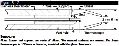
A probe consisting of a Pitot tube containing a thermocouple (Figure 5.12) and systems to minimize losses by conduction and radiation can be used to measure the stagnation temperature. Despite the best planning procedures, the probes will still read a temperature lower than stagnation temperature and, unfortunately, the correction varies appre­ciably with temperature, the Reynolds number and the Mach number.

Heat losses are in general: 80% by conduction and radiation from the shield, 15% by conduction from the base, 5% for conduction through the thermocouple wires, but they can change dramatically with changes in the design of the probe. The effectiveness of such a probe is usually defined on the basis of a recovery factor, r, given by:

Tm – T T – T2

where Tm is the measured temperature. The following conditions will apply:

■ Shape of the probe: The chamber has an opening in the front for the thermocouple and ventilation holes immediately downstream of the thermocouple. The walls of the chamber are mirrors to reduce heat losses by radiation from the junction of the thermocouple.

■ Temperature sensor: Any thermocouple capable of withstanding the temperatures to be measured can be used. The junction should be far away from the support so as to leave a long section of the wires exposed to hot air to reduce losses by conduction. The heat capacity of
the junction should be as small as possible to reduce the response time of the probe.

■ Anti-radiation shield: An anti-radiation shield must surround the temperature sensor. The temperature of the shield is different from that of the sensor and therefore the temperature measured is influenced by heat transfer by radiation. To minimize this effect, the shield must have low conductivity, like the silicon shield in Figure 5.12, and the surface must be a mirror. The effectiveness of the shield can be enhanced by heating it or by using multiple shields (up to five).

■ Ventilation holes: As the air temperature in the stagnation chamber of the probe tends to decrease, due to conduction and radiation, it is necessary to provide vent holes to continuously replace the air in the chamber. When it is necessary to measure temperature fluctua­tions, the exchange of air helps in not damping fluctuations. The best ratio between area of the holes and entrance area of the probe, AV/A is a function of heat loss and should still be small so that air does not assume appreciable speed. Usually this ratio varies between 0.2 and 0.4.

■ Effects of Reynolds and Mach numbers: The presence of a normal shock wave at the entrance of the probe does not alter the value of the stagnation temperature. Obviously the performance of the probe deteriorates with increasing temperature (increasing losses due to all types of heat transfer): Figure 5.13 illustrates the typical decrease of

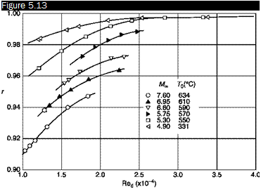Effects of Reynolds and Mach numbers on the recovery factor of a stagnation temperature probe

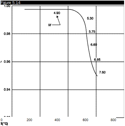
the recovery factor with decreasing Reynolds number and with increasing Mach number. Figure 5.14, derived from the data of Figure 5.13, shows the rapid decrease of the recovery factor that occurs when the Mach number exceeds the value 5. It can be concluded that in a supersonic wind tunnel (M < 5), a probe with a single shield has a recovery factor very close to 1 if the Reynolds number of the probe is greater than 20,000. For hypersonic wind tunnels (M > 5), probes can be made more accurate using small heating elements and thermocouples in the base of the probe, with additional heaters and thermocouples on the inner side of the shield. This will provide heating to balance the losses: in practice, the base is heated until it reaches the

Probe for measuring the stagnation temperature: decrease of the recovery factor with temperature and Mach number

Source: [4]

Note: Red = 20,000. Probe with a single screen

same temperature as the main thermocouple and subsequently the shield is heated until its internal temperature is equal to that of the thermocouple. After another balancing all the temperatures are equal and the losses by conduction and radiation are zero (recovery factor equal to one).

A non-dimensional expression of the film coefficient h [/m-2s-1] should be used, for example the Nusselt number (Nux = hx/l) or the Stanton number (St = Nux/RexPr), because numbers can be conveniently expressed in terms of other characteristic numbers. For example, for a flat plate in a gas stream (Pr и 1):

Nux = 0.332(Rex) (Pr) laminar boundary layer

Nux = 0.0296(Rex) (Pr) turbulent boundary layer

By the change of Nusselt number with the abscissa, the transition from laminar to turbulent regime can be determined. The measurement of h can be made with an unsteady method.

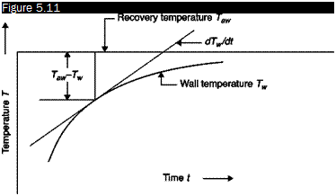
In a hypersonic flow, a body, which initially is at room temperature, undergoes aerodynamic heating, the temperature rises very quickly at the beginning then more and more slowly as the difference between the wall temperature and the adiabatic (or recovery) wall temperature decreases. If the model is made with an insulating material, the temperature of each point of the model tends asymptotically to the value of the local adiabatic wall temperature (Figure 5.11).

If the wall temperature is measured with a thermocouple using the technique in Figure 5.2, with the wall made of an insulating material, it can be assumed that all the energy exchanged by convection through the metal disk of area A goes to increase the internal energy of the metal plate to which the thermocouple is welded. The coefficient of heat transfer by convection, h, can be obtained from the unsteady energy balance:

qA = hA AT aw – Tw) = mcd – h= me dTwldt

A Taw – Tw

Determination of the coefficient of heat transfer by convection with the unsteady method

where m is the mass of the disk, c the specific heat of the wall and dTJdt the slope of a plot Tw (t) obtained in the measurement (Figure 5.11).

When the flow is not hypersonic, this technique can be still applied, up to Mach numbers close to zero, by a prior heating or cooling of the body with respect to the stream temperature. For M ^ 0, static temperature coincides both with the stagnation temperature and with the adiabatic wall temperature.

Transition from a laminar to a turbulent boundary layer can be detected by the increases in adiabatic wall temperature and/or film coefficient. These methods are additional to those listed in Chapter 6 (visualization methods, optical methods), to the measurement of stagnation pressure at
a fixed distance from the wall or to the measures of turbulence in the boundary layer with anemometers (Chapters 3 and 4).

5.1.1 Measurement of the temperature recovery factor

The adiabatic wall temperature is usually expressed in a non-dimensional form, temperature recovery factor, r, defined as the ratio between the actual rise in temperature of the adiabatic wall with respect to the static temperature of the stream (Taw – TJ, and the temperature rise that would occur if the flow were stopped isoentropically (T0„ – TJ. The temperature recovery factor can be expressed in terms of the Mach number, the adiabatic wall temperature and the stagnation temperature as follows:

The recovery factor depends only on the Prandtl number, Pr = Cppll where Cp [/Kg-1^-1] is the specific heat at constant pressure. The Prandtl number is a measure of the relative importance of the dissipation of kinetic energy due to the dynamic viscosity, m [Kgm-1s-1], and the heat conduction due to the coefficient of conductivity, l [/K_1m-1s-1]. In the boundary layer the viscous stresses tend to increase the local temperature to a greater extent when the shear rate is strongest (near the wall), the conductivity creates a heat flow toward the colder areas (furthest from the wall) which makes the temperature near the wall to decrease. For gases, which have Pr < 1, the second effect is more important than the first one, therefore the resulting adiabatic wall temperature is lower than the stagnation temperature.

Equations linking the recovery factor to the Prandtl number are different according to the regime of flow, laminar or turbulent. For a flat plate:

r = VPT in the laminar regime,

r = -^PT in the turbulent regime

Because, for air, Pr < 1, the recovery factor is higher in the turbulent than in the laminar flow regime usually passing through a maximum in the region of transition.

If the transition from laminar to turbulent boundary layer occurs, there are conditions for non-uniform wall temperature on the body and heat flows from the turbulent zone to the laminar zone, leveling out the temperatures (the brass wall in Figure 5.8). In order to measure the true adiabatic wall temperature, care must be taken to minimize the effects of conduction along the wall: the model must therefore be made of an insulating material (the lucite wall in Figure 5.8).

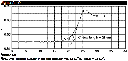
Since the position of the transition, namely the critical Reynolds number, depends also on the intensity of turbulence of the incoming stream, sometimes to determine the quality of a supersonic or hypersonic wind tunnel transition cones are used with apex angles of 5° or 10°. The procedure consists of measuring the critical Reynolds number for the whole range of Mach numbers and Reynolds numbers of the wind tunnel and comparing the data obtained with those of similar wind tunnels. Then it can be decided if additional turbulence screens or other modifications of the wind tunnel are needed.

Figure 5.8

1

о

ф

2

э

25

ф

о.

Е

,ф

Source: [1]

Schematic of the transition cone JPL

Source: [2]

To apply this technique, the cone should have:

■ dimensions such that local Reynolds numbers between 2 x 106 and 7 x 106 can be generated on the surface;

■ low heat capacity;

■ very accurate surface finish.

The cone of Figure 5.9 is hollow and made of fiberglass, except the tip that is made of steel. Thirty copper-constantan thermocouples are arranged on the surface at intervals of 2 cm. The surface is covered with several layers of plastic coating, straightened and painted.

The cone is calibrated in an oven to check that all the thermocouples are working and that their readings are uniform. Once inserted in the wind tunnel and the test has been carried out, the readings of the thermocouples are converted into temperature recovery factor, r, by Equation (5.1). The typical result of a test is shown in Figure 5.10. In the first part of the cone, where the flow is laminar, the temperature recovery factor has a value of about 0.85, in transition a maximum value of about 0.894 is attained and finally it stabilizes at the turbulent value (0.886).

Determination of the critical Reynolds number in a wind tunnel with a transition cone

x(cm)

It should be noted that there is not unanimity in the choice of the characteristic length to be used in calculating the critical Reynolds number. The different methods can lead to variations of l + 2 x 106 in the calculation of Recr.

The surface temperature of opaque bodies can be calculated by measuring the intensity of the emitted radiation which increases with the fourth

power of the body temperature. The range of wavelengths involved (Figure 5.5), l = 0.45 – r – 100 pm, goes from the visible, 0.45 – r – 0.75 pm (high temperatures), to the infrared (down to temperatures below ambient temperature).

This type of measurement overcomes some of the difficulties typical of diagnostic methods discussed in the previous paragraphs:

■ no alterations of the surface of the model is induced;

■ the sensitivity is in the order of tenth of K.

The relationship between the temperature of an object and the radiation received by the detector depends on the emissivity of the surface and on the absorption of the optical system: for each model and for each type of test, a prior calibration is therefore needed, for example, using thermocouples embedded in the surface of the model.

In the measurements with infrared camera, both optics and windows of the wind tunnels are critical because glass and quartz cannot be used, being both opaque to infrared radiation. Lenses are usually made of expensive germanium; cheaper materials quite transparent to infrared radiation are lucite, silicone and Domopak film.

The sensors used are indium antimonide (InSb), sprite (HgCdTe), lead selenide (PbSe), covering the field 2 – r – 13 pm: these are therefore suitable for measuring temperatures from 200 K to 2000 K (with appropriate filters). Since the sensitivity of these sensors increases when their operational temperature decreases, they should be kept at temperatures well below ambient. The different techniques used are:

■ cooling with liquid nitrogen at about 80 K; liquid nitrogen is difficult to maintain for a long time, not more than 2 hours, so the system is reserved for fixed installations in scientific laboratories;

■ cooling to 90 K by expansion of compressed argon (Joule-Thomson effect); the argon can be kept easily in cylinders and, unlike liquid nitrogen, its consumption is zero when the thermograph is not used;

■ cooling to 70 г 90 K with a Stirling pump which, in a closed circuit, compresses and expands helium; the circuit needs to be recharged only after a few thousand hours, the system is therefore suitable for field measurements;

■ cooling to 200 K with a thermoelectric (Peltier) circuit (thermocouple, in which a potential difference is applied and a temperature difference between junction and reference is obtained), the system is particularly suitable for surveillance cameras on a continuous basis.

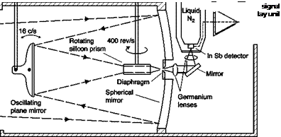
If only one sensor is used, it is necessary to send on it in succession signals from each point of the field, i. e. a mechanical scanning of the image is needed. In Figure 5.6, an image of the field is produced by a spherical mirror of 200 mm diameter oscillating 16 times per second around a horizontal axis combined with a prism rotating at 400 revolution/second around a vertical axis; horizontal and vertical scanning, respectively, are performed in this way and the infrared radiation from each pixel is focused in turn on a single indium antimonide (InSb) sensor. The sensor converts thermal radiation into an electrical signal that is used to modulate the intensity of the beam of a cathode ray tube: the vertical position of the beam is synchronized with the position of the oscillating mirror and the horizontal position is synchronized with the rotating prism, each pixel of the field is thus transformed into a corresponding

Schematic of AGA thermograph ThermoVision 750

— Vertical sync, signal

— Horizontal sync, signal

Cam

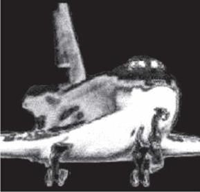
Thermographic image of a space shuttle in a hypersonic wind tunnel

pixel of the video screen. With this system, 16 images per second can be obtained.

To increase the frequency of images, multiple sensors can be used arranged in a row to eliminate the vertical scanning: with 10 – r – 30 sensors and a rotating polygon with 8 – r – 10 faces 30 images per second can be obtained. The most recent version of the camera provides in the focal plane of the objective a matrix of 320 x 240 uncooled microbolometer (768,00 pixels): 60 images per second are obtained. The resolution of the cameras is about 0.1 K, the error is of the order of 2% or 2 K (the larger of the two values).

The thermographic image of a model space shuttle in a hypersonic wind tunnel is shown in black and white in Figure 5.7.

The temperature of a body can be measured by using temperature-

sensitive paints, and these may be, in order of increasing performance:

■ phase-change paints whose basic component is a wax: an isotherm is identified by the line of separation between the solid and liquid phases. With these paints, it is only possible to identify areas of the body that are at temperatures below or above the melting temperature of the wax; the coating can be used only once.

■ multi-component paints: each component undergoes a color change at a specific temperature and hence each isotherm is identified by a line of separation between two different colors. In the areas between two isotherms, it can be argued that the temperature is between the two values. The color change is irreversible, so the coating can be used only once.

■ a reversible color change can be produced with a coating of liquid crystals. Temperature changes alter the molecular structure of these crystals causing a change in the wavelength, and then in the color, of the scattered light.

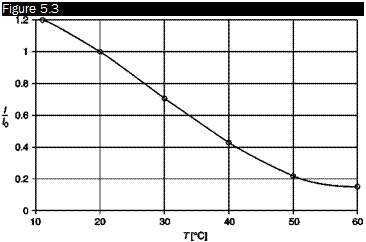
■ temperature-sensitive paints (TSP) are fluorescent elements (pho­sphorus), analogous to the pressure-sensitive paints, which, stimulated with an appropriate radiation, emit light whose intensity decreases with temperature (Figure 5.3); the emitted light is of a wavelength

Typical dependence of the light intensity emitted by a TSP on temperature

different from that of the exciting light, for example (Figure 5.4), a paint excited with ultraviolet light (280 г 390 nm) emits red light (580 г 630 nm). This feature makes it possible to filter the incident light and measures only the emitted light. Paints have been developed to measure temperatures ranging from ambient up to 1000°C.

The application of the method is subject to some restrictions:

■ The thermal properties (emissivity and heat transfer) of the surface can be altered by the coating.

■ The need to work in a darkroom or with low light imposes restrictions in applications, but ambient light, as well as exciting light, can be filtered out.

■ The response times of phosphorescence to changes in temperature are important in the study of transient phenomena, they differ greatly from one paint to another but are low enough for phosphorus of the type ZnS-CdS. With a moderately strong ultraviolet excitation, such as that produced by a mercury arc lamp, it is suggested that the response time is less than 0.3 s.

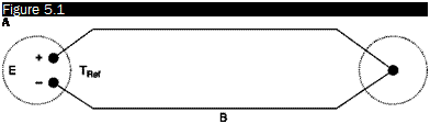
Any two wires of different metals A and B can be used as a thermocouple if connected as in Figure 5.1. When the temperature of the junction, Tjct, is different from the reference temperature TRef, a weak potential difference, E, is generated at the terminals +/-.

The value of E depends on the materials A and B and on the difference between reference temperature and junction temperature:

E=T (a-z)T

J yRef

where eA and eB are the thermoelectric power or Seebeck coefficients of the two metals.

For small temperature differences, the following linear equation can be used:

E = (єА – Єв){Т"}а — TRef ) = £AB (T]a — TRef)

where eAB is the Seebeck coefficient of the couple of metals.

Schematic of a thermocouple

The three most common thermocouples are copper-constantan (type T), iron-constantan (type J) and chromel-alumel (type K): the first element of the couple is positive, the negative wire is coded with the red color. All three types are available in pairs of coated wires with a minimum diameter of 25 pm. For reasons of accuracy and space, the minimum diameter possible should be chosen taking into consideration that wires with a diameter less than 75 pm are very weak.

■ Copper-constantan (type T, color codes: blue and red): eAB и 40 pV/K, Tmax = 300°C. Neither wire is magnetic. Junctions can be obtained by welding or brazing with usual welders.

■ Iron-constantan (type J, color codes: white and red): eAB и 50 [pV/K], Tmax = 650°C. Iron is magnetic. The junction can be obtained by welding or brazing with usual welders. The couple iron-constantan can generate a galvanic electromagnetic force: it cannot be used in the presence of water.

■ Chromel-alumel (type K, color codes: yellow and red): eAB и 40 pV/K, Tmax = 1100°C. Alumel is magnetic. The junction can be obtained by welding or brazing with silver, at the higher temperatures iron must be used. This couple generates electrical signals when subjected to deformation.

To measure higher temperatures the following thermocouples may be used:

■ Platinum-platinum/rhodium: Tmax = 1650°C

■ Iridium-ruthenium/iridium: Tmax = 2100°C

■ Tungsten-tungsten/molybdenum: Tmax = 3200°C.

Thermocouples can be purchased ready-made or can be made in the laboratory from pairs of wires using a specific thermocouple welder or any suitable welder for fine wires.

The reference temperature can be controlled in several ways:

■ melting ice is widely used in laboratory because it is accurate and inexpensive: a thermos can maintain 0°C for several hours if filled with crushed ice and water;

■ systems are available that provide reference temperatures controlled electronically; these devices are not as stable as melting ice, and require periodic calibration but are very easy to use;

■ other instruments use as a reference the temperature that is generated within the container, assuming that this is not affected by environ­mental conditions;

■ in less accurate measures the room temperature can be used as a reference.

The main difficulty encountered in the use of thermocouples is the need for the junction and the wires not to disturb the temperature distribution in the wall. It is advisable to check the effect of the thermal conductivity of the wires and the heat transfer to or from the junction to determine the measurement error in each individual application:

■ In a metal wall, the junction can be welded directly to the metal, taking care not to alter the character of the surface and its emissivity. The simple method of welding the junction to the surface and spreading out the wires parallel to the surface in an isothermal layer, to minimize losses by conduction, can be adopted only in incompressible flows; such a system, causing shock waves in supersonic flows and disrupting the surrounding boundary layer, would completely alter the local temperature conditions: in this case, the sensor should be placed inside the body.

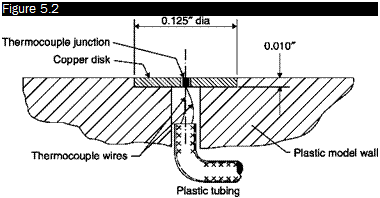
■ With models made of insulating material good results can be obtained by using discs of copper or silver, approximately 3 mm in diameter and 0.25 mm thick, inserted into the wall flush with the surface. Figure 5.2 shows this arrangement of the thermocouple used for measurements in a supersonic field: the disk can easily reach the temperature of the surface and quickly follow any change in temperature due to its low heat capacity. The influence of radiation can be reduced by covering the insert with a thin layer of lacquer having an emissivity similar to that of the wall.

Measurement of temperature of a plastic wall with a thermocouple

Abstract: This chapter highlights both contact temperature sensors (thermocouples and temperature sensitive paints) and devices allowing measurements of temperature at a distance: infrared thermo-cameras. Devices and techniques used to measure tempera­ture recovery factor, film coefficient and stagnation temperature of an air stream are described.

Key words: infrared thermo-cameras, temperature sensitive paints, thermocouples.

5.1 Sensors

Temperature measurements are of great importance in problems of heat transfer between a body and a fluid stream. If the flow is incompressible, the only relevant temperatures are the wall temperature, Tw, and the static temperature of the stream, TM. In supersonic and hypersonic flows aerodynamic heating is present and it is necessary to consider also the stagnation temperature of the stream, T0m, and the adiabatic wall temperature, TaW.

Temperature sensors can be classified into two main groups: contact sensors and remote sensors. Among the contact sensors thermocouples are dominant in point measures, temperature-sensitive paints (TPS), are used with success in the mapping of large areas.

In order to obtain reasonably accurate measures of temperature with contact sensors, some basic requirements must be fulfilled:

■ as every sensor measures its own temperature, it is necessary that the sensor be in thermal equilibrium with the body;

■ the sensor must not conduct heat to or from the point of measurement;

■ the probe should not interfere with the way in which heat transfer occurs between the stream and the body: conduction, convection, radiation and mass transfer (evaporation or condensation); for example, if there is radiation, the emissivity of the wall should not be modified by the presence of the sensor.

The remote sensors deduce the temperature by measuring the radiation, infrared or visible, emitted by the body: the measure is not limited to high temperatures (pyrometry in the visible), efficient methods have been developed (thermographic cameras) which allow the measure in the infrared range, even at temperatures below ambient, with an accuracy comparable to that of a thermocouple.

Time resolved PIV technology is currently available, which obtains 4000 images per second, adding the dimension time to the measures of a fluid – dynamic field. With CTA, LDA and L2F techniques, the behavior in time of speed at a single point could be obtained. The study of the structures present in the stream was delegated to the methods of visualization. The missing element was the combination of spatial information derived from the PIV with the simultaneous history of each point. The next step is time resolved PIV, providing a more thorough examination of the fluid dynamic phenomena and the correlation time-space. The results (Figure 4.37) are similar to those obtained by computational fluid dyna­mics using large eddy simulation.

Succession of images of velocity and vorticity fields obtained in real time