Category Aerodynamics of a Lifting System in Extreme

The so-called PARAWIG works as a sail wing in proximity to the ground. It is common knowledge that the main distinction of a sail compared to a rigid wing is that its surface is subject to deformation under the action of the flow, and the difference of the pressures on pressure and suction surfaces of the sail is proportional to its longitudinal curvature. According to Twaites[186], the problem of the aerodynamics of a sail consists of determining the flow for a given incidence в and excess of length S = ls — 1, where ls is the length of the sail.5 Essentially, this implies predicting the form of the sail wing, the aero­dynamic loading and the tension on it. To solve for the flow, the conventional equation of the wing theory has to be supplemented by a condition of static equilibrium of each element. Naturally, the resulting system of equations is different from the traditional formulation for a rigid wing. One of the specific results of sail theory is the theoretical possibility of the existence of more than one form of sail for prescribed в and 5. However, there is no difficulty in choosing a real form. For such forms it turns out that the lift coefficient Cy of the sail exceeds Cy of the rigid wing approximately by the value of 0.636y/S. In what follows, we analyze very simple mathematical models of a PARAWIG in the concrete case of a flexible foil of infinite aspect ratio in the extreme ground effect. Fortunately, in this particular case, Twaites’s [186] verdict “…An analytical solution seems out of the question ” is not true. A complete linearized formulation for the perturbed velocity potential of a steady flow past a thin flexible foil near the ground can be written as

d2<p dV

dx2 dy2 ’ = y = h±0’ <12’46>

— = »-*• <12^

|?=0, у = 0 + 0, (12.48)

V(p —> 0, x2 + y2—> oo. (12.49)

Equation (12.47) accounts for the interaction of a flexible foil with the flow field and means that the pressure difference across the wing is proportional to the longitudinal curvature, and the factor of proportionality is the ten­sion T.

Again, all lengths are related to that of the chord.

Applying the asymptotic approach advocated in this book for vanishingly small ground clearances /г —> 0, we can derive the following simplified formu­lation for a PARAWIG in a steady two-dimensional extreme ground effect flow:

(12.50)

d^ii = 1 f&y

dx 2 dx2 ’

For a flexible wing, the ordinates у of the foil camber line with respect to the flat ground can be written as

y(x) = h + Ox + rj(x),

where 77 (x) represents the deformation of the wing due to the aerodynamic interaction with the flow, 77(0) = 77(1) = 0.

Integrating the first of the equations (12.53) and using the Kutta – Zhukovsky condition 7(0) = 0 for x = 0, y(0) = h, we obtain

Combining (12.54) with the second equation in (12.53), we obtain the follow­ing equation with respect to r/(x):

77" + a2r] = —6a2 x,

where

The solution of this equation was found in the form

rj = C cos ax + C2 sin ax — Ox.

Equations for determining the constants follow from the requirement that the deformation vanishes at the edges of the foil. Then,

?y(0) = Ci = 0, 77(1) = Ci cos a 4- C2 sin a — 9 = 0,

Finally, the deformation function rj(x) is obtained in form of the expression , 4 „/sinax , 4 rj(x) = в ————— x. 12.55 sin a / The excess length, which should be equal to J, can be calculated as Employing the smallness of 0 and, consequently, y’ = 0(0), x ; 1 #2 f1 ( 2cos2(ax) А i> s = is-i = – f fl2.2; ; -1) ae Л Jo sin (ax) / sin 2a >

a* / sin 2a 1 2 ( -^ “I—- о— ) 2 sim a V 2a / J

Cl = 0, c2

Now, we turn to calculation of the lift coefficient of a PARAWIG in the two dimensions and in very close proximity to the ground:

~ о f1 /v о 0/sinax

Cy = 2 j(£)d£ = 2 tx+t[———————— x)

Jo Jo La a sin a )

For a small relative excess length, we can express the lift coefficient in terms of S —У 0, the angle of pitch, and the relative ground clearance h:

(12.59)

The relative effect of the flexibility of the foil can be evaluated by relating expression (12.58) for the lift coefficient of soft foil to that for a rigid foil (T = oo, a = 0). Eventually,

Figure 12.2 illustrates the relative variation of the lift coefficient of a flexible foil versus the combined parameter 5/в2.

Essentially, the approach applied above suggests that the tension in the foil is sufficiently large Th = 0(1). It can be seen that at certain (eigen) combinations of the tension parameter and the relative ground clearance unstable modes occur of flow past a flexible lifting surface. Examining a homogeneous problem for deformations 77 of the foil,

r?" + a2T) = 0, ф) = 0, 77(1) = 0,

it is easy to conclude that the eigenvalues of the product Th are[78]

(Th)n = —Д-~, n = 1,2,…

By using the previous relationships, we can calculate the eigenvalues for the elongation 5 versus the form number n.

The corresponding eigen forms are described by expression

What are the relationships between the amplitude of a certain harmonic and the elongation parameter <5? Suppose that the amplitudes of the eigen forms of a foil are designated as rj0ri so that accounting for a — nn, the equation of the nth form becomes 77 = r]0ri sin7rnx. Then the elongation parameter S can be expressed as

5 = ls — 1 ~ ^ f (nnr]0ri)2 cos2 rmxdx = ^-‘K2n2riln,

2 Уо 4 n

so that for the nth harmonic, the amplitude will be related to the elongation 5 by

2V~5

The corresponding lift coefficient СУп will be

c-=ll sin”“di=^[ i-(-i)”i-

For even forms n = 2m(m = 1,2,…), the corresponding contribution СУп to the lift coefficient is zero.

For odd forms n = 2m — 1 (m = 1,2,…),

r = 4г?02т_х = 8л/б

У2т-1 7г/і(2ш — 1) /і7Г2(2ш — І)2 *

If we include all harmonics in the expression for the form of the foil, then,

oo

v(x) = ХЖ sin тгпх,

П— 1

where у = h + Ox + rj and rj(0) = rj( 1) = 0. In terms of the vortex strength 7 and foil ordinates у measured from the fiat ground surface, the set of governing equations becomes

5x(y7) = 5x’ 1 – (! -7)2 = – Ту", y = y{x).

Integration of the first equation of (12.63) and accounting for the Kutta – Zhukovsky condition 7(0) = 0 for x = 0, у = /г, gives

У

Substituting the previous result in the second equation of (12.63),

1 – % = – Ту".

yl

Multipying the latter equation by yf,

y’ – h2 = – Ty’y"

or and integrating, we obtain the expression

h? T., „

y+J = ~2y +C’

where C* is a constant to be determined later. Resolving with respect to y’,

2 z’ /i2>

or

/(C*-y-h?/yУ To determine the constant C* of integration we impose the conditions of no deformation at the edges of the wing, 2/(0) = h, y( 1) = в + h, wherefrom follows the equation for determining C* rh+0

у/C* — у — h2/y

(12.64)

Introducing parameter a = у/2/Th, we can write (12.65) and (12.66) in al­ternative forms:

x _ 1 fy___________ dy_______ o = f1+e______________ dу_________

aJi y/(C* – у – 1/y)’ Л /(C* – y-l/y)’

with ^ С* = С*//г, and 0 = 9/h.

The tension parameter T is defined by the condition of a prescribed elon­gation of the length of the foil:

(12.67) which together with equation (12.66) enables us to find the relationship be­tween elongation and tension. Note that the slope of the foil contour yr in the equation for S has to be expressed through C* and y. The lift coefficient of a PARAWIG in the nonlinear case is determined by straightforward integration of the pressure jump across the foil:

cy= [ l{x)[2-~f{x)dx = -?[у'(1)-г/(0)] = (12.68)

Jo a

VC* – 2h

C* – h – 9 –

i. e., to the leading order the lift coefficient of a flexible foil is completely deter­mined by the slopes of the foil contour at the edges. Performing calculations, we obtain

The notion of a flexible wing as a sail brings us to the consideration of an important property of a sail – porosity. Twaites [186] indicates that the lift – to-drag ratio for a sail is relatively small, partly due to porosity. Porosity is known to diminish the lift. The through flow due to porosity is assumed to be proportional to the pressure jump. For a porous flexible foil moving in immediate proximity to the ground, the governing equations have the form

where a(x) > 0 is a nondimensional porosity factor.

In the linearized 2-D case, the governing system (12.70) yields

Assuming a = const, and eliminating 7 from the previous expressions, we obtain the following ordinary differential equation with respect to the у or­dinates of a porous flexible foil:

y’" + 2p" + ^V = 0. (12.72)

Representing у = h – f Ox – P T](x), where rj(0) = rj( 1) = 0, we can write the following equation with respect to the perturbation of the form of the foil

ф):

rl" + 2^t/’ + a? r{ = – а2в, a = a/h, a=y^- (12.73)

Although implicitly such a formulation implies that a = 0(h), it will be assumed that a is sufficiently small in comparion with the relative ground clearance. Investigation of eigen solutions of a homogeneous equation corre­sponding to (12.72) leads to the following expression for the relative speed of divergence:

(12.74)

where da is a dimensional porosity factor and C0 is the chord of the foil. From observation of (12.74) we can conclude that the porosity of flexible foil entails a delay in the occurence of instability.

[1] This means that a cost-effective ocean-going vehicle capable of handling high seas should be sufficiently large. On the other hand, a vehicle of small dimensions is expected to be efficient on inland waters, where high seaworthiness is not required.

[2] This parameter represents the ratio of the distance of a wing from the ground to the chord of the wing and later on will be called the relative ground clearance.

[3] It can be shown that an infinite number of regular parameter expansions can be derived around h = oo, providing different ranges of validity with respect to h.

[4] E. Tuck seems to have been the first to introduce the term extreme ground effect, widely used in this book; see also Read [51].

[5] Extension to compressible flow will be considered in 5.1.

K. V. Rozhdestvensky, Aerodynamics of a Lifting System in Extreme Ground Effect © Springer-Verlag Berlin Heidelberg 2000

[6] In the steady case, this parameter coincides with the relative ground clearance h measured at the trailing edge.

[7] near the trailing edge /2,

[8] Here notation h stands for the characteristic relative ground clearance.

K. V. Rozhdestvensky, Aerodynamics of a Lifting System in Extreme Ground Effect © Springer-Verlag Berlin Heidelberg 2000

[10] For a wing with a straight trailing edge, xte = 0.

[11] Flow tangency conditions on the upper and lower surfaces of the wing:

[12] Parabolic arc

Let the foil have the form of a parabolic arc with relative curvature Sc. In this case, f(x) = 4x(l — x), a

[13] Strictly speaking, the theory of a wing of small aspect ratio implies that the local span increases monotonically in the downstream direction.

[14] With an asymptotic error of the order of 0(h).

[15] Note that the case under consideration corresponds to the order relationship 0 – C ol "C h – C 1, complying with the assumptions of linear theory: both the relative ground clearance and the angle of attack are small, and the latter is always smaller than the former.

[16] Coefficient of the moment around the leading edge:

[17] This conclusion correlates well with an exact solution of the problem of the optimal wing; see de Haller [134].

[18] To the order of 0[h, hln(l/h)}.

Note that in this formulation the ground clearance is measured from the trailing edge of the flap.

[20] As previously, this terminology implies that the maximum relative thickness is of the order of the relative ground clearance h. This assumption is practical and allows analyzing the influence of the thickness up to 10-15% of the chord.

[21] It may, for example, incorporate the factor of the contraction of the flow leaking from under the endplate.

[22] The assumption of the ideal fluid separation scheme on the flap is adequate for the power augmentation mode at rest. It can also be considered practically adequate for the cruise mode in a pronounced ground effect due to the domination of the channel flow contribution.

The “hats” are taken off.

[24] Energy equation

K. V. Rozhdestvensky, Aerodynamics of a Lifting System in Extreme Ground Effect © Springer-Verlag Berlin Heidelberg 2000

[25] If, for example, a wing in compressible flow has an angle of attack a, then the

angle of attack of the equivalent wing becomes a! — a/ y/l — Mq.

[27] Here instead of the notation for pitch 6, we use a.

[28] Far from the endplate on the lower surface of the wing (y —> —oo, у = 1—0),

[29] The ground clearance is measured between the hinge of the flap and the unper­turbed position of the ground surface.

[30] Here, the reactive component of the lift coefficient is substracted from the total lift coefficient.

[31] i) It is common to assume that due to the very small ratio of densities of air and water, the surface under a lifting system in the ground effect behaves as if it were solid, ii) The assumption of stillness of the wavy boundary implies that the speeds of propagation of sea waves are small compared to the cruising speed of a wing-in-ground-effect vehicle. It is not difficult to introduce the effects of wave speed into the model.

[32] As earlier, all lengths are related to the root chord of the wing.

K. V. Rozhdestvensky, Aerodynamics of a Lifting System in Extreme Ground Effect © Springer-Verlag Berlin Heidelberg 2000

[33] For Lw = 2, the wave is two times longer than chord of the wing.

[34] The same is true for any wing with a flat lower surface moving in the extreme ground effect.

[35] Note that in the Appendix the longitudinal moment coeffcient mZw was also calculated around the trailing edge.

[36] Practically, this mode of motion takes place when the vehicle’s pitch is kept fixed

by controls.

[38] The minus derivative of the cruise lift coefficient with respect to the ground clearance can be interpreted as the “stiffness” of the spring in a simple mass­spring model of a vehicle on a dynamic aircushion.

[39] For large waves the height-to-wave ratio constitutes approximately 1/20.

[40] For a wing-in-ground-effect vehicle flying over the sea surface, this assumption is reasonable. It follows from the statistics of sea waves that the velocity of progressive waves does not exceed 1 knot, whereas the speed of existing and future wing-in-ground-effect vehicles varies in the range from 50 to 300 knots.

[41] Another argument exists in favor of this scheme based on some data showing that the magnitudes of drag, obtained in theory, are somewhat larger than the experimental ones.

[42] For the practical situation of blowing turbulent jets this result does not hold because due to certain momentum losses related to jet impingement upon the ground, the decrease in the averaged jet velocity and the entrainment of the surrounding air causes an increase in the jet width in the downstream direction.

[43] This case was considered by Gallington et al.

[44] As designated earlier, Л is the aspect ratio of the wing and 5ep is the characteristic relative gap under the endplates.

[45] Note that this and other quantities that may vary spanwise are assumed to be averaged in the lateral direction.

[46] In fact, the same rate of leakage from under the endplates allow for different combinations of the width of the effective gap under the endplates, the wing’s aspect ratio and the relative ground clearance.

[47] Based on a reentrant jet model.

[48] Most of the practical foil families have analytical descriptions.

[49] This is valid in a wide practical range of Strouhal numbers.

In the reentrant jet scheme the role of such a model parameter is played by the angle of inclination of the jet with respect to the downstream direction.

[51] This formula assumes that the wing is flat and the tips of the endplates are parallel to the ground.

[52] In the sense of minimal induced drag.

[53] The length of the plate is equal to that of the wing’s chord.

[54] Note that this formula does not include viscous pressure (form) drag and, con­sequently, gives a very approximate estimate of the viscous drag.

[55] That is, the lift coefficient, corresponding to the maximum aerodynamic effi­ciency.

[56] This can be achieved by using endplates with sharp tips or keels with sharp tips fixed on floats.

[57] That is to reduce the magnitude of the lift coefficient, corresponding to the maximum lift-to-drag ratio.

[58] The term was introduced by A. N. Panchenkov [64].

K. V. Rozhdestvensky, Aerodynamics of a Lifting System in Extreme Ground Effect © Springer-Verlag Berlin Heidelberg 2000

[60] The integrodifferential equation of the lifting line for an unbounded fluid can be found in Ashley and Landahl [161].

[61] C(z) is a ratio of local chord to the root chord.

[62] In Munk’s sense, i. e., ensuring minimal induced drag for a given lift.

[63] Note that for a parabolic planform, Л = 3//2.

[64] In the literature one may often encounter the alternative term ram in association with the ground effect.

[65] Note that for span-dominated and chord-dominated ground effects, the optimal planforms of the wings are different, although both give rise to a parabolic dis­tribution of loading.

[66] If the lift coefficient is kept constant, while the wing approaches the ground, the induced drag coefficient decreases in both models of extreme ground effect.

Again, with the reference area equal to half that of the tandem.

[68] Matters of automatic control are covered in Diomidov [179].

[69] Incorporating both viscous and induced drag.

[70] This is valid for small relative distances of the wings of the tandem from the ground.

[71] All quantities and functions are rendered nondimensional by using the chord

length Co and the speed of forward motion U0.

K. V. Rozhdestvensky, Aerodynamics of a Lifting System in Extreme Ground Effect

© Springer-Verlag Berlin Heidelberg 2000

[75] In the case when the flutter is possible.

[76] It is possible to demonstrate that introduction of small porosity augments the speed of divergence; Efremov [71].

[77] Note that structural damping is not accounted for here.

[78] See also paragraph 12.2, dedicated to the approximate prediction of the occur­rence of instability on an elastic foil under the action of tensile forces.

Efremov [70]—[72] was one of the first to analyze at length important matters of the static and dynamic aeroelasticity of a lifting surface in proximity to the ground. We consider first a wing of infinite aspect ratio. Then, in the
case of static aeroelasticity, the elastic deflections of the foil contour can be determined by the simplified equation

f, i‘I – dV _ +

da?-tm=v ~P

with boundary conditions (for a freely supported plate)

m-m-gm-gw-*.

where T is the stretching longitudinal force, T = 2T/pU„C0 and p~ — p+ is the nondimensional pressure difference across the foil, causing its deformation f(x).

We consider an infinitely thin foil in the extreme ground effect. Recalling the material of section 3, we can formulate the following (linear) problem for determining the pressure difference (aerodynamic loading) p~ — cor­responding to the flow past an elastic foil with a distribution of ordinates ys(x) = y0(x) + /(x), where y0(x) characterizes the basic configuration of the foil and /(x) gives the perturbed displacements of points on the foil due to elasticity:

where (рг is the perturbed velocity potential in the channel flow.

It is assumed that in the course of elastic deformation, the end points of the foil (leading and trailing edges) remain in the same positions, i. e., 2/s(l) = 2/o(l) and ys(0) = y0(0) or, in other terms, /(0) = /(1) = 0. Representing the perturbation velocity in the channel flow as a sum

dK _ <H dyi,

dx dx dx

with terms corresponding to the basic foil configuration and its perturbation, we can integrate (12.22), accounting for the Kutta-Zhukovsky condition, to obtain

= [Vo(x) – 2/o(0) + f(x),

wherefrom

(12.24)

Now, it is possible to replace the right-hand side of equation (12.19), using expression (12.24). The resulting equation has the form

D— – T— – -/ = 0.

dx4 dx2 hJ

Determination of the condition of the occurence of the static instability of an elastic foil can be reduced to finding eigenvalues of a two-point homogeneous boundary problem, comprising equations (12.25) and (12.20). First, we con­sider particular cases. For D = 0, we deal with a membrane foil, and the corresponding stability equation takes the form

Т~л + / = °> (12.26)

The eigenvalues and eigen forms of the foil that comply with problem (12.26),

(12.20) can be easily found to be

ATn = (^Т/Г) =ШГ’ fn(x) = sin гига:. (12.28)

As seen from this result, the loss of stability of a membrane foil occurs at a certain critical speed, whose minimal magnitude can be associated with the speed of divergence UQd. Relating the speed of divergence to the quantity y/T/pC0, which also has a dimension of speed, and setting n = 1, we can derive the following expression for the nondimensional speed of divergence

UQd:

U0d = ^== = 7rVh. (12.29)

Up* VWpc!

v^Y pCо

Another concrete case can be obtained for a purely elastic foil when T = 0,D ф 0. In this case, the divergence condition can be deduced from the equation •D. 2 f — о dx* d/ “ II II Q Ipu2co3 V hD (12.30) and (12.20) in the form Ad„ = п2тг2, (n = 1,2.. ■), (12.31)

Deriving eigenvalues for the more general equation (12.25), rewritten in the form

7Г*

(12.33) It is easy to see that in particular cases when D = 0,T ф 0 and and T = 0,D ф 0, expression (12.33) yields the previous results of (12.29) and (12.32). Comparison of (12.33) and (12.32) indicates that when an elastic foil is subject to the action of stretching tension (T > 0), the loss of static sta­bility occurs at higher speeds.[76] It is important to emphasize that for h —> 0, the speed of divergence of elastic foil is proportional to the square root of the relative ground clearance. An analysis of the mathematical model of dynamic aeroelasticity with the pronounced effects of lag both in terms of aerodynamic loads and elastic deflection in the extreme ground effect leads to the following generalized equations of free (eigen) oscillations of a flexible foil in the vicinity of solid ground:[77]

and subject to conditions (12.20), we obtain the following formula for the relative speed of an divergence of elastic foil under tension:

4>h (x> t) = Фі (x) exp(ikt), f(x, t) = f(x) exp(ita), (12.36)

where к = ujCq/U0 is the Strouhal number, і = >/“ї and eliminating px from the previous two equations, we obtain the following homogeneous ordinary differential equation of the sixth order with respect to f(x):

(12.37)

Taking f(x) — /о ехр(ірж), p = П7Г, we obtain the following characteristic equation:

Dpe + Tp4 – 2^—5tk2 + хУ + ^ + X = O’ (12‘38)

It is convenient to rearrange equation (12.38) as a quadratic equation with respect to the eigen magnitudes of the Strouhal number к:

ijs‘+1k)k2-jk~ Л0*’+- D=■<12’39»

Solving this equation for к = kn, we obtain

(12.40)

The minimal magnitude of the speed U0, which turns the expression under the square root into zero, can be associated with speed of flutter; see [71]. The resulting expression for the relative (minimal) speed of flutter U0t can be found from (12.40) for n = l, p = p = 7Г in the form

One can see from equation (12.41) that the speed of flutter diminishes as the relative ground clearance tends to zero. The Strouhal number fcf, corresponding to the flutter condition, is given by the expression

To a certain extent, the asymptotics of the extreme ground effect furnish an analog of the “piston theory” and permit us to evaluate the magnitudes of the critical speeds.

In a similar fashion, we can analyze the static stability of a wing of finite aspect ratio in motion close to the ground. For example, following the lines of the approach discussed above, the problem of the membrane wing in flow is reduced to the problem of the stability of a flexible plate subject to the action of tensile forces. In the latter case, the problem of eigen solutions is governed by the equation

– 9 d2f

Taaf+hd‘° (1243)

and corresponding boundary conditions. An analysis of the dynamic stability of an elastic lifting surface can be carried out on the basis of the equation

DAAAf – TAAf – 2—6tk2Af – + + Щ-j – 0, (12.44)

p h h ox h

where / = /(x, z) is a complex function of two independent variables.

Efremov also examined the influence of compressibility upon the charac­teristics of flexible foils. It was shown that at supersonic speeds the flexibility of the foil can give rise to an additional wave drag. In the case of subsonic flexible foil at small distances from the ground, a differential equation was obtained, describing the complex interaction of longitudinal elastic waves of deformation and acoustic waves in the gas.

Herein, the definition of a flutter will be restricted to that of a phenomenon of oscillatory instability of an elastic wing in a potential flow without separation or shock waves. The essential feature of flutter is a certain interaction of the degrees of freedom of an elastic wing, entailing the influx of flow energy to this wing.

In a simple mathematical model of the flutter of a wing in the extreme ground effect, the analysis will focus on the interaction of two degrees of freedom related to elastic heave and pitch oscillations in a two-dimensional flow past a flat plate. To evaluate the speed of flutter, we write equations of the free elastic oscillations of foil in nondimensional form as

fi(h + кЩ – Су – цв(хе – xcg),	(12.2)
/і Іе(0 Ч – &$$) = Tflz ^/l(Xe *Ecg)?	(12.3)

where p = 2M/pSC0 = 2M/pCq • 1 represents the density of the ’’vehicle”, ге = іK; ie is the moment of inertia of mass calculated with respect to the elastic axis, i. e., the point whose abscissa x = xe; xcg is the abscissa of the center of gravity, and kh = u>hC0/U0 and ke = w>eC0/U0 are Strouhal numbers, based on circular frequencies and associated with heave and pitch springs, which model two elastic degrees of freedom of the foil. Representing pitch and heave motions as harmonic oscillations,

6{t) = 0O exp(ikt), h(t) = h0 exp(ikt), (12.4)

where к = ujC0/U0 is the Strouhal number based on circular frequency и of oscillations and і = л/-Л, we can find the lift and the moment (around the abscissa xe of the elastic axis) coefficients Cy and mz by using solutions of the corresponding problems presented in paragraph 3.5. Heave-related coefficients were determined in the following form:

Cyh(t) = j-Ahexp(ikt), Ah = – 4k, (12.5)

m*h = exp(ikt), Bh = B£ – Ahxe, = fc(5fc 8г), (12.6)

where h is the relative ground clearance, measured from the trailing edge of the foil.

The lift and the moment coefficients for pitch oscillations can be found by the following formulas:

)*-xt

г2 г3 у 2 *^е

where

Substituting the expressions for 6(t) and h(t), as well as the heave and pitch contributions to the lift and moment coefficients, we can write the following system of homogeneous equations with respect to the amplitudes в0 and h0 of the oscillations:

[Ah + Mhfc2(l – Kl)]h0 + 0o[Ae + Mhk2(xe – rrcg)] = 0, (12.10)

[Bh + fihk2(xe – xcg)]h0 + в0[Вв + /ih*efc2(l – «h«eh)] = °- (12-n)

Note that the system written above contains a combined parameter рь = that can be called the reduced density. This parameter was initially introduced in the analysis of dynamic stability; see section 11. The parameters «h and Kffh represent ratios of circular frequencies

a>h xi в

— 5 К eh —

UJ U>h

where cj represents that of free oscillations.

The critical condition of flutter is reached for a combination of Kh and к = loC0/U0, or for a given wing, for a combination of the circular frequency cj and the speed of forward motion f70, when the determinant of the ho­mogeneous system of equations becomes equal to zero. The magnitude of U0 corresponding to the critical condition of flutter may be defined as the speed of flutter and will be designated as Uf. Composing the determinant Л of the system and equating it to zero, we obtain the following equation for determining fth and fc, corresponding to flutter:

A{kh, k) = [Ah(fc) + цьк2( 1 – «£)][£*(*) + Vhiek2(l – K-Weh)}

~[Ae(k) + /uhfc2(xe – xcs)][Bh(k) + nhk2(xe – leg)] — 0.

It is worthwhile mentioning that A is complex-valued. Therefore, setting the determinant to zero means equating to zero both its real and imaginary parts, i. e., ША = 0 and ЭЛ = 0. The latter equations enable us to determine two real quantities «ь and k. It can be seen from the structure of the flutter equation, written above, that it can be rearranged into a quadratic equation with respect to /С =

a(k)K? + 2 b(k)K + c(fc) = 0, (12.14)

where the coefficients a(fc), b(k), and c(k) are complex-valued functions of the Strouhal number k, given by the formulas

a(k) = a3a5^h, c(k) = (a2 + a3)(a4 + a5) – ab

b(k) = -^[a3(a4 + a5) + ^ha5(a2 +a3)], where a, i = сц(к),і = 1 • • • 5 are written below:

ai(fc) = [Ah(k) + /іьk2(xe – xcg)][Bh(k) + /іьk2(xe – scg)], a2(k) = Ah(k),

a3(fc) = /ihfc2, a4(fc) = Bg(k), a5(fc) = /іьгеА:2.

Separating the real and imaginary parts in (12.14), we obtain the following two equations with respect to JC =

Ua(k)JC2 + 2 m(k)K + Щк) = 0, 2 Щк)К, + Qc(k) = 0. (12.15)

-m(k) ± ^m[75](k) – Щк) ~ Щк)

Selecting the appropriate root of the quadratic equation and equating it to the solution of the linear equation, we can solve the resulting relationship2 with respect to к = kf and, consequently, find the corresponding magnitude of /С = /Cf = Then the speed of flutter Uf can be determined in the

The first of these equations with real-valued coefficients is still quadratic, whereas the second is linear in JC. The solution with respect to /С is straight­forward

Equation (12.17) enables us to evaluate the speed of flutter for a given circular frequency u>h of the heave spring and the chord length C0 of the foil. For similarity considerations it is convenient to form a nondimensional speed of flutter Uf. This can be done by relating Uf to the quantity uj^Cq which has the dimension of speed. The resulting expression can be written as

Some calculated results for the two-dimensional flutter of a flat plate in the extreme ground effect are presented in Fig. 12.1 in form of a graph, showing the behavior of the nondimensional speed of flutter versus the reduced density /ih = fih for different ratios of the circular frequencies of the pitch and heave springs tt<9h = ujq/uj^. These results correspond to the following magnitudes of input quantities: xe = 3/4, xcg = 2/3, ie = 1/18. One can observe from the graph that for a considered a decrease in the reduced density /іь leads to a diminution of the speed of flutter. It is remarkable that in the extreme ground effect, the influence of the relative ground clearance h and the density of the wing /і, which are combined in just one parameter /іь, are somewhat similar. For example, the same relative reduction of either h or (i entails an identical drop in the speed of flutter. If the same wing flies closer to the ground, its speed of flutter becomes smaller, i. e., the proximity of the ground reinforces flutter-related restrictions upon the speed of the vehicle as compared to flight in unbounded air.

The elasticity and flexibility of the lifting surface can play a particular role in ground-effect aerodynamics due to the expected increase of dimensions of wing-in-ground-effect vehicles, use of light materials and fabric, etc. Usually, to account for elastic properties and/or flexibility of the wing, we have to consider simultaneously the equations of aerodynamics and elasticity. In a more profound analysis, the formulations should also cover the equations of the dynamics of the vehicle. As a relationship, linking the deformations of a lifting surface with aerodynamic loading, we normally use equations of unsteady bending of an elastic plate accounting for forces, acting in its camber plane; see Bisplinghoff et al. [151]. In nondimensional form,[71] [72] [73] [74] this equation can be written as

2JS‘U + + + =*- -J>+- <12-»

The following notations are used in (12.1) for functions and parameters: / are vertical displacements of points of the elastic plate, pw is the density of the material of the plate, p is the density of air, 5t is the thickness of the plate, D = 2D/pUqCq, D is the bending (cylindrical) stiffness, Nxx and Nzz are factors that characterize the forces acting in the x and z directions, respectively, Nxx – 2Nxx/pU%C0, and =

Equation (12.1) should be solved with boundary conditions, correspond­ing to the method of fixing the edges of an elastic and/or flexible lifting surface, as well as with initial conditions that define the initial magnitudes of the deflection and the rate of deflection of the surface.

The formulations for an elastic/flexible wing can be used both for eval­uating the variation in aerodynamic properties due to the deformation of the lifting surface and for predicting the occurence of static (divergence) and dynamic (flutter) instability. In what follows, some simplified schemes are considered for analyzing conditions of the aeroelastic instability of a wing in the extreme ground effect. The last paragraph contains approximate predic­tions of the influence of the flexibility of the foil upon its lift coefficient and some effects of the porosity of a soft foil.

One of the parameters relevant to the design of wing-in-ground-effect vehicles is the so-called binding criterion; see Zhukov [175]. The binding criterion enables us to foresee what would be the behavior of the vehicle in height and pitch with variation in the speed of longitudinal motion. In what follows some simple quasi-static considerations will be used to relate the derivatives of the ground clearance and pitch with respect to speed to such characteristics as the static stability margin, the position of the center of mass, the magnitude of forward speed, the lift coefficient and its derivatives with respect to height and pitch; see Rozhdestvensky [182].

Suppose that the vehicle operates in a cruise mode in a state of static equilibrium with regard to vertical displacement and rotation around the lateral axis that passes through the center of mass. In this case the following equations of equilibrium hold:

Mg^Cy^-S, Mz = mz^SCo = 0. (11.60)

Z Z

2U0 dU0Cy + U* dCy = 0, 2U0 dU0mz + U* dmz = 0. Writing out the full derivatives with respect to height, we obtain Expressing the total derivatives by partial ones,

(11.61) (11.62) (11.63) (11.64) dh ah ‘ дв dh~ dh~n ‘ de~*dh’ (1L65) Then, it follows from (11.62) and (11.63), taking into account (11.64) and (11.65), that

OTT dU0 2/ auy d(Jydd Ж. ж*,с, + UQ (х, ж = 0

0TTdU° n ^TT2( 0(Jy, dUydU 2U° dh Xc*Cy + u° Xh dh +Хв дв dh)~ °- Substracting (11.67) from (11.66), we derive

where M is the mass of the craft, g is the acceleration of gravity, Cy is the lift coefficient, U0 is the cruise speed, Mz and mz are the longitudinal moment around the center of gravity and its coefficient, respectively, p and S are the density of air and the wing reference area. Differentiating equations (11.60), we obtain

2U0^Cy(xe – xcg) + C/2(xg – *h)^ = 0,

wherefrom follows the first binding criterion (for height)

dh 2U0Cy /xCg xq 2U^Cy /xCg ~~ xq

dU0 Cg x9-xh) Cg xh-xe)’

with

It can be easily seen that the binding criterion for pitch can be obtained from that for height by a simple substitution h -> в and в —)• h:

It follows from observation of the binding criteria (11.69) and (11.74) that for a statically stable vehicle, the location of the center of mass has a direct effect upon the response of the vehicle to an increment of speed or a horizontal gust of wind. Suppose that the vehicle is designed so that the abscissa of the center of mass coincides with the abscissa of the center of height xcg = Xh – In this case, as seen from (11.69) and (11.74), it will respond to an increment in speed by an increment in height without a change of pitch. On the other hand, if the center of mass coincides with the center of pitch xcg = x#, then the vehicle is expected to change pitch angle due to the variation in speed while flying at the same height. This consideration shows that by a thorough selection of the reciprocal locations of the three important centers (center of mass, center in pitch and center in height), one can provide static stability to the vehicle and also render its motion control system more efficient.

An option for securing the longitudinal stability of a wing-in-ground-effect craft consists of using the tandem scheme with both wings operating at small relative ground clearances.

The parameters of the front and aft wings of the tandem should be se­lected to provide an appropriate stability margin. Owing to the fact that the interaction effects of small clearances are of the order of О (/г), one can perform a qualitative analysis of the stability of a tandem foil configuration based on the aerodynamics of a single foil in extreme proximity to the ground. Here some results are presented of an analysis of the static stability margin of a tandem foil configuration (Л = oo) for the particular case when the foils have equal chords and ground clearances hi = /12 = h = 0.1. In the calcula­tions, the center of gravity of the tandem was assumed to coincide with the trailing edge of the front foil. The distance between the foils constituted 20% of the chord.

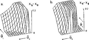
Figure 11.6a depicts the magnitude of the static stability margin versus the adjusted pitch angles (related to the ground clearance, i. e., #1,2 = #1,2/h) of the front and rear foils when both foils are flat. We can conclude upon examination of this figure that, whereas a single foil is not statically stable, addition of another foil can result in a positive static stability for certain combinations of adjusted pitch angles. It can also be observed from Fig. 11.7a that for better stability it is advisable to put more loading upon the front foil [185].

The static stability of longitudinal motion for a tandem can be further enhanced by curving the lower surface(s) of one (or both) foil(s). Fig. 11.6b reflects the increase in the reserve of the static stability of the tandem when the front foil has a sine type curvature with amplitude s = 0.2h — 0.02.

A simplified analysis of the influence of the design parameters on the position of the characteristic centers and the static stability of a tandem

Fig. 11.6. 3 – D charts of the static stability of a tandem comprising two foils versus their adjusted pitch angles related to the ground clearance hi = /12 = h: a. both foils are flat, b. front foil has a sine curvature.

configuration can be conducted within the linear theory of a foil in in extreme ground effect; see chapter 3. Assuming that the wings of the tandem are flat, have identical chord lengths C0, and an infinite aspect ratio, we can derive the following formulas for the abcissas of the center of pressure (жр), the center of height (rch)> and center of pitch (xg):

P — Xp Ls 1.

In these formulas the following notations have been introduced: Cyi and Cy are, respectively, the lift coefficients of the front wing (based on its ref­erence area) and the tandem as a whole (based on the sum of the reference areas of the front and rear wings); Ls is the distance of the trailing edge of the front wing from the leading edge of the rear wing, related to C0; and = /12 f h, i. e., the ratio of the relative ground clearance of the rear wing to that of the front wing. Introduction of the lift coefficient of tandem as a whole is practical for the analysis because for a selected wing loading and cruise speed, the vehicle should be designed for a fixed magnitude of the cruise lift coefficient.

Observation of the formula allows us to draw some preliminary conclusions about the position of characteristic centers in the case under consideration. In particular,

• when design ground clearances of the front and rear wings are indenti – cal,3 the center of height coincides with the center of pressure xh = xp. As per Zhukov[175], the closeness of these centers to each other improves controllability of the vehicle; see also 11.2.3,

• in the case under consideration, for fixed magnitudes of the lift coefficients of the front wing and the tandem as a whole, the position of the center of pressure does not depend upon the ratio /12/^1-

Based on the analytical results presented above, the simplified analysis of the stability is reduced to a calculation of the positions of the three char­acteristic centers and the static stability margin SSM = xh — xg versus the parameters Cyi, Cy, Ls, and /%. The results of some calculations are pre­sented in Figs. 11.7-11.11.

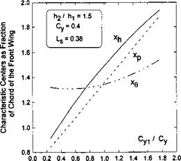
Figures 11.7-11.9 exemplify the effect of the ratio of the design ground clearances /12/^1 of the tandem wing elements upon the dependence of the positions of the characteristic centers on Cyi/Cy. One can conclude from observation of these graphs that by varying the design ratio of the ground clearances of the front and rear wings of the tandem, we can bring the cen­ter of height to different positions coincident with the center of pressure, upstream or downstream of the center of pressure.

Fig. 11.9. The calculated relative abscissas of the aerodynamic centers of a tan­dem craft versus the lift coefficient of the front wing as a fraction of the total lift coefficient, /12/hi = 1.5.

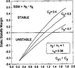
Fig. 11.10. The calculated static stability margin SSM = Xh~ x$ of a tandem craft versus the lift coefficient of the front wing as a fraction of the total lift coefficient, h2//ii = 1,LS = 0.38 for different magnitudes of the total lift coefficient.

Figures 11.10 and 11.11 show more explicitly whether the vehicle is stable and what is the dependence of its static stability margin SSM = — xq on

different design factors. In all cases the calculations confirm a conclusion of [185] that for better static stability, it is desirable to put more load­ing onto the front wing. Figure 11.10 shows that (for a fixed fraction of the front wing loading) reducing the lift coefficient of the tandem brings about the deterioration of static stability. In practical design terms this means,

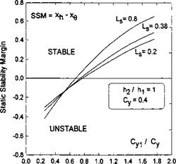
Fig. 11.11. The calculated static stability margin SSM = Xh — xg of a tandem craft versus the lift coefficient of the front wing as a fraction of the total lift coefficient, h2/h = 1 ,Cy = 0.4 for different magnitudes of the spacing between the wings of the tandem.

for example, that for a prescribed speed of the vehicle, a reduction of wing loading may lead to a lower reserve of the static stability.

Figure 11.11 illustrates the effect of the spacing between the wings of the tandem. The conclusion here is straightforward: enlarging the distance between the wings entails augmentation of the static stability margin.

A question may arise why the tandem, even with flat (identical) wing elements can be designed to be statically stable, whereas an isolated single wing shows neutral static stability, see 11.2.1. A reasonable answer to this question is if the wing elements of the tandem secure height stability, the whole system acquires pitch stability.[70]

h*2(x) ’

1 f1 xdx 2 J0 h*2(x) ’

We consider first a simple example of a single foil at a full rear flap opening. As follows from (4.92), for Jf = 1 the lift and the moment coefficients of a single foil in the extreme ground effect are given by the formulas

where h is the relative ground clearance defined at the trailing edge. Writing h*(x) as h*(x) = 1 + Ox + ef(x) (where 6 = 6/h, є — є/h, and є = 0(h) is a small parameter that characterizes the curvature of the lower surface of the foil ), we can differentiate (11.47) with respect to h and в to obtain

It follows from (11.48) and (11.49) that the quantities hCy, hCy, hmz, and h mz depend upon 0 and є rather than upon 0, /г, and e. In accordance with the assumed order relationships of the small parameters, this means that the above quantities are of 0(1). Most important is that the number of defining parameters is fewer by one (in this case 2 instead of 3). Now we can determine the position of the centers of height and pitch in the following fashion:

Note that according to (11.47), both the lift and the moment coefficients in the two-dimensional extreme ground effect depend on the similarity param­eters 0, є, i. e., Cy = Су(в, є) and mz = тг(в, є). Hence, the derivatives with respect to height and to pitch can be obtained in an alternative form:

c»‘==-№i+cis)’ ”»=4H5+m’?)- <n-52>

Cy 21 h* re ___ 2 Ґ f(x)dx У Jo h*3

0 f1 x2 dx = Jo T*"’ _ _0 f1 xf(x) dx Jo h** ‘

Using (11.50)—(11.52), we can write the following alternative expressions for the abscissas of the centers of height and of pitch:

We can be conclude from (11.53) that for a flat plate (e = 0), the abscissas of the centers of height and of pitch coincide. Hence, a flat foil in the ex­treme ground effect is neutrally stable. However, (positive) static stabil­ity of a single foil can be achieved by introducing a nonplanar (curved or/and polygonal) lower surface to the foil. It follows from the extreme ground-effect theory that the aerodynamic response of the flow depends on the local dis­tribution of the width of the channel under the wing

h*(x) = 1 + 6x + £/(x),

where h*(x) = /і*(х)//і, в = 0//i, and є = є/h, and £ is a parameter of the curvature of the lower surface of the foil. This means, in particular, that the stability margin of a curved foil depends upon the ratio of the curvature to the ground clearance rather than upon the curvature proper. It follows therefrom that to ensure the same reserve of stability for smaller ground clearances, one has to turn to proportionally smaller curvatures.

As discussed earlier in this section, one of the known recipes for im­proving stability of a single foil is S-shaping; see Staufenbiel and Kleinei – dam [177], Gadetski [183], etc. A simple representative of such a family is a foil with a sinusoidal lower surface described by the form function f(x) = — sin(27rx), x Є [0,1]. It turns out that other forms of the lower surface can be proposed which also lead to the enhanced static stability of the longitudinal motion, see Rozhdestvensky [185].

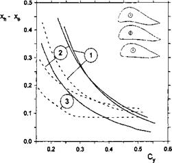
In Fig. 11.1a comparison is presented of the behavior of the SSM = x^—xq versus the design lift coefficient for the previously mentioned sine foil, a special stab foil whose equation for the lower surface is f{x) = —15x(l — x)5 and a delta foil, whose lower surface is composed of two flat segments joined in a vertex located at 25% of the foil chord from the trailing edge. For the latter foil, the form function that characterizes the curvature of the lower surface can be written as

Fig. 11.1. Static stability margins for foils (Л = oo, h = 0.1, solid lines) and rectangular wings with endplates (Л = 0.625, h = 0.1, 8°p = 0.025). The numbers correspond to 1: “sine” foil section; 2: “stab” foil section; 3: “delta” foil section.

In all calculated cases, the ratio of the curvature parameter to the relative ground clearance was є = 0.2, which corresponds to maximum curvatures of the lower surface is equal to є — eh — 0.2h. The tentative geometries of the sections of the aforementioned three foil types (number 1 corresponds to the sine foil, number 2 to the stab foil, number 3 to the delta foil) with thickness distribution of NACA-0008 on top of the corresponding lower surface and appropriate rounding of the leading edge are also shown in Fig. 11.1 for the design ground clearance h = 0.1. To better demonstrate the form of the foils, the vertical dimension is multiplied by 4.

Plotted in the same figure are some calculated results for rectangular wings of finite aspect ratio Л = 0.625 for the same foil sections, ground clearances, and relative curvatures. The gap under the endplates was assumed to be 5°p = 0.025. Figure 11.1 shows that for a wide range of variation of the lift coefficient, the increase in the degree of three-dimensionality (an augmentation of the gap under endplates) brings about a deterioration of the static stability, although qualitatively the behavior of the static stability margin versus the cruise lift coefficient is similar to that of the 2-D foil. Note that, based on the results of their theoretical calculations, Staufenbiel and Kleineidam concluded that the way of shaping the foil for better static stability has a similar effect on a rectangular wing with a modified airfoil section.

Figure 11.2 shows the static stability margin of a 2-D foil with a sinusoidal lower surface versus the cruise lift coefficient and for different ratios of є/h. Figure 11.3 presents an estimate of the influence of position x& of the delta foil upon the position of the center of pressure xp, the center of pitch xq, and

the center of height x^. Figure 11.4 illustrates the dependence of the positions of the aerodynamic centers of the delta foil upon the ratio в/h of the pitch angle to the relative ground clearance. In Fig. 11.5 some calculated data are plotted, showing the effect of a short rear flap upon the static stability margin. In particular, it follows from Fig. 11.5 that even a small blockage of the flow near the trailing edge leads to noticeable diminution of the static stability margin. This is quite natural because once the flow underneath the foil stagnates, the form of the lower surface has almost no influence upon

Fig. 11.5. The influence of a short trailing edge flap on the static stability of a delta foil in the extreme ground effect, є/h = 0.2, Xd = 0.2.

the aerodynamics. A conclusion that follows from these results is that if the static stability of longitudinal motion of the vehicle is secured by profiling the lower surface of the wing, control by a rear flap should be applied with caution.

One of the difficult points in the design of lifting systems in the ground effect is to provide a sufficient margin for the static stability of longitudinal motion.

As shown by Irodov [166], Kumar [167], Staufenbiel [177], and Zhukov [171], the longitudinal static stability of the motion of a wing-in-ground-effect ve­hicle depends on the reciprocal location of the aerodynamic centers of height and of pitch. The reserve of static stability also depends on location of the center of gravity. We define positions of the aerodynamic centers of height and pitch, respectively, as

where the superscripts h and в are ascribed, respectively, to the derivatives of the lift and the moment coefficients with respect to the ground clearance and the angle of pitch. Through analysis of the linearized equations for the longitudinal motion of wing-in-ground-effect vehicles, Irodov [166] showed that static stability is ensured if the aerodynamic center of height is located upstream of the aerodynamic center of pitch, so that for x axis directed upstream, the corresponding static stability criterion can be written as

Xh – Xg > 0.

For the coordinate system adopted in this book, with x axis directed upstream, the formulation of the condition of the static stability of longitudinal motion, used by Zhukov and Staufenbiel, implies that the full derivative of the lift coefficient with respect to the ground clearance (for a fixed zero magnitude of longitudinal moment around the center of gravity) should be positive, i. e.,

Essentially, the latter inequality shows that for a statically stable vehicle, the stabilizing effect of dCy/dh should exceed the destabilizing influence of nose-down moment. Note that Zhukov designated the full derivative of the lift coefficient with respect to the relative ground clearance as a force stability pa­rameter and pointed out that this factor has an effect upon the controllability of the vehicle and its response to the action of wind. For a properly designed vehicle, the derivative dCy/dh should be negative, and we can rewrite (11.42) as

(11.43)

It can be seen from (11.43) that Irodov’s criterion deals with pitch stability, implicitly assuming that height stability is provided, i. e., Су < 0, whereas the criteria of Zhukov and Staufenbiel represent the combined effect of pitch and height stability.

We designate the above difference in the location of the aerodynamic centers as SSM = x^ — xg and, when SSM is positive, we refer to it as to the static stability margin. Suppose that both derivatives (of height and
of pitch) and the positions of corresponding aerodynamic centers are defined with respect to a certain reference point, say, to the trailing edge. In practice, they have to be defined with respect to the center of gravity which can be viewed as a pivotal point. Introducing the abscissa xcg of the latter and noting that changing the reference point does not affect differentiation with respect to h, whereas

d_ d__ d_

дв дв Xcgdh’

we obtain the following formulas for the new positions of the centers of height and of pitch (when the reference point coincides with the center of gravity) expressed by corresponding parameters referred to the trailing edge:

where /С = CyjСу. For a foil that possesses height stability and Су/Су < 0, factor /С is negative. It may be practical to evaluate the variation of the static stability margin as a function of the position of the center of gravity (the pivotal point). Simple calculations lead to the following equation:

= (®h – xe) -> SSMcg = – A_SSM. (11.46)

It can be seen from (11.45)-( 11.46) that if a wing is found to be statically stable with reference to the trailing edge, its static stability is ensured for any other upstream position of the reference point (center of gravity), see Irodov [166]. A wing that is statically unstable with reference to the trailing edge remains statically unstable for any other position of the reference point. Si­multaneously, equation (11.45) shows when the center of gravity is shifted upstream from the trailing edge, the center in pitch moves in the same di­rection, whereas the center in height retains its position. Consequently, the static stability margin diminishes.

At present several optional aerodynamic configurations of wing-in-ground – effect vehicles are known that enable us to secure the static stability of longitudinal motion. In a wing-tail combination, employed in Russian first – generation ekranoplans, the main wing operating in close proximity to the underlying surface was stabilized by a highly mounted tailplane, taken out of the ground effect. This measure shifted the center of pitch downstream, thus increasing the static stability margin for a practical range of design pitch angles and ground clearances. The negative effect, associated with the use of a large nonlifting tail unit consists in an increase in structural weight and a noticeable reduction of the lift-to-drag ratio.

Another possibility is connected with the use of a tandem aerodynamic scheme with both lifting elements located close to the ground. When de­veloping his first З-ton piloted SM-1 prototype, Alekseev borrowed a tandem configuration from his own designs of hydrofoil ships; see Rozhdestvensky and Sinitsyn [19]. Jorg [7, 8] applied a tandem configuration in the design of his “Aerofoil Flairboats.” Note that to provide static stability to a configuration comprising two low flying wings, one has to adjust the design parameters of these wings (pitch angles, relative ground clearances, and curvatures of pressure surfaces of the wings) in a certain way. The shortcoming of a tan­dem as an option in providing static stability of longitudinal motion to a ground-effect vehicle, consists of a somewhat narrow range of pitch angles and ground clearances for which the flight is stable [22].

A way to reduce the area of the tail stabilizer (or to get rid of it) is related to appropriate profiling of the lower surface of the main wing. It means that instead of a wing section with an almost flat lower surface, known to provide a considerable increase in lift in proximity to the ground, one has to give preference to wing sections with curved lower surfaces which secure static stability, although are less efficient aerodynamic ally. Staufenbiel and Kleineidam [177] proposed a simple way to augment the static stability of the Clark-Y foil with a flat lower surface, which consists of providing this foil with a trailing edge flap, deflected to an upward position. Later on, the same authors found that if unloading of the rear part of the foil is combined with decambering of its fore part, the range of static stability can be enhanced noticeably. A family of foils with an S-shaped mean line may be shown to possess such a property. In their stability prediction for an S-shaped foil, Staufenbiel and Kleineidam [177] used an approximation of the foil’s mean line with a cubic spline function. The parameters of this curve fitting function were selected to provide the maximum range of lift coefficient in which the foil would be stable. An experimental investigation of the influence of the form of the airfoil upon its static stability was carried out by Gadetski [183]. Based on his experimental data, the author concluded that it is possible to control the positions of the aerodynamic centers by proper design of the foil. He demonstrated experimentally that an upward deflection of the rear part of the foil moves the center of height upstream and the center of pitch downstream. A similar investigation using the method of conformal mapping and an experimental technique of fixed ground board was done by Arkhangelski and Konovalov [184].

In what follows, a qualitative analysis will be carried out of the static longitudinal stability of schematic aerodynamic configurations by using the mathematical models of the extreme ground effect, see Rozhdestvensky [185]. The simplest case involves a wing of infinite aspect ratio moving in immedi­ate proximity to the ground. In this case, within the assumptions of extreme ground effect aerodynamics, it is possible to determine the characteristic centers, whose reciprocal positions define both the static stability and the
controllabity of the configuration, in analytical form. The effect of the finite aspect ratio is estimated by applying the nonlinear one-dimensional theory of a rectangular wing with endplates in motion close to the ground. A study of the static stability of a tandem configuration of infinite aspect ratio is made, assuming that for h 0, the foils constituting the tandem work indepen­dently.

11.1.1 Order Estimates and Assumptions

We turn to the evaluation of the form of the quintic equations of motion for h —> 0; see Rozhdestvensky [181]. In section 4, order estimates were obtained for the major aerodynamic coefficients on the basis of a mathematical model of a simple flying wing configuration in immediate proximity to the ground. In particular, for an adjusted angle of pitch (in radians) and a curvature of the wing sections of the order of 0(h),

Cyo, mzo= 0(1), CXiQ = 0(h). (11.25)

As per the previous analysis, the derivatives of the aerodynamic coefficients have the following order of magnitude:

(Cy, mz)h^ = 0(1), (11.26)

С’шё = o(i). (11.27)

Additionally, we assume that the viscous drag of the configuration does not vary with a small variation in the ground clearance and the pitch angle. To evaluate the order of magnitude of the coefficient Cf7, which represents the derivative of the thrust coefficient with respect to the relative speed, it is assumed that the drop of the thrust versus the cruise speed is linear, so that the (current) thrust T of the engines can be expressed in terms of the relative speed of motion, installed thrust Tm and cruise thrust T0 as

T = Tm-U(Tm – T0), £/ = yp (11.28)

b’o

where U0 is the design cruise speed. Introducing the thrust coefficient as

2T 2Tm U 2(Tm — T0)

‘ pUfS pUiS U0 рСуаЩв ’

wherefrom the derivative of the thrust coefficient with respect to the relative speed is given by

s-iU _ 2(Tm — T0) _ 2Cyo(Tm — T0) _ /Tm To

* “ PU*S ~ pCyoU*S – yovw w)

= -Cyo (cTm -^-)=CX – CyoCTm, (11.29)

where Crm = Tm/W is the installed thrust-to-weight ratio that characterizes the relative power capacity of the vehicle.

Recalling previous order estimates and assuming additionally that the installed thrust-to-weight ratio Crm = 0(h),

c? =Cx-CyoCTm=0(h). (11.30)

It seems rational to consider the magnitude of yt as that of the order of O(h). In other words, the ordinate of the thrust line is assumed comparable with the ground clearance.

Another convention to be adopted is related to the density factor p that enters the equations of motion. Based on the statistics for existing and pro­jected wing-in-ground-effect craft (see Rozhdestvensky [182]) we can assume that the product of the vehicle’s density and relative ground clearance is of the order of 0(1). In this case, it is appropriate to introduce, instead of /z, a new quantity p^ = p h = 0(1), which can be called the reduced density.

11.1.2 Asymptotic Form of the Equations of Motion for h —ї 0

Employing these estimates and conventions about the orders of magnitude (in terms of h) and neglecting terms of the order 0(h) and higher, we can reduce the equations (11.18)—(11.20) to

Mh^-=0, (11.31)

d2h – і ~ ~

Ph ^2 — al h ~h h ~b G-з в – f – 0-4

d20 ^

Ph iz ~^2 — h T b2 h + Ьз в + 65 #,

where ai = hCy, a2 = hCy, a3 = hC^, a4 = hCy, and ph bi (i = 1,2,3,4) are given by the formulas

61 = hmj, b2 = hmhz, 63 = hmGz, 64 = hm9z.

Note that coefficients ai and bi are of the order of unity, because for each of the above derivatives,

coefficient^’^ = O^-j.

The system of equations (11.32) and (11.33) has a structure similar to that of equations (11.9) and (11.10), derived on the basis of Irodov’s assumption

of no perturbation in speed. It gives birth to a quartic characteristic equa­

tion (11.11) whose coefficients are identical to А*, і = 1… 4, though written somewhat differently:

A =———- т(Ьа ~b iz ^2)? (11.35)

A2 =—————————– ^“7“ [&4 b2 – a2 64 + flh (63 + izdi)], (11.36)

lz

As = —2^(a2 — CL4 b — as b2), (11.37)

Mh lz

A4 = -^r-(ai b3 – a3 6i). (11.38)

Mh lz

The advantage of the formulation presented above consists of the reduction in the number of parameters on which Ai depend. In par­ticular, for h —> 0, the relative clearance h does not enter the coefficients of the quartic equation explicitly. Thus, the coefficients of the quartic depend (nonlinearly) only on the reduced density цh and ratios є/h that characterize the design geometrical and kinematic parameters of the vehicle. The parame­ter є = О(h) can be the adjusted angle of pitch в or the maximum curvature c of the lower surface of the wing related to /г, etc.

The variation of speed can be analyzed by introducing “large time” t = 0(1 /К) and “very large time” t = 0(1 /h2). It can be shown that on the scale of a “large time,” the variation of the speed of the vehicle is mostly driven by perturbations in height and pitch, whereas on the scale of “very large time” the variation of speed is determined by the perturbation of speed proper. In the latter case, the perturbed equation for speed is completely uncoupled from those for height and pitch and has the form

= -2CX)U’,

where t2 = h2 t is a “squeezed” time variable and /h and Cx = Cx/h

are quantities of the order of unity.

If we account for the perturbation of the speed of the forward mo­tion, the corresponding equations can be written as

=(Ct° -2C*o)w – as – a-h – cej – ckx (11.18)

d[69]h • ~ • •

^ = 2 U’Cyo + Ceye + Ceye + Chyh + C$h, (11.19)

(i2n _ ….

= Vt(2CX0 – C?)U’ + meJ + mhzh + mhzh + meJ. (11.20)

In these equations, U’ represents the relative perturbation of the cruise speed, Cf is a derivative of the thrust coefficient with respect to the relative speed of forward motion, Cx is a static drag coefficient,2 and yt is the vertical distance of the thrust line from the vehicle’s center of gravity. As earlier, all quantities are rendered nondimensinal using the cruise speed U0 and the root chord C0. The drag coefficient is related to the instantaneous cruise speed U0(l + Uf). Excluding two of the three unknown parameters, we obtain the following fifth-order (quintic) characteristic equation of the perturbed system:

HD – (Cf – 2CXn ) CtD + СЇ Ф + Свх

-2 Cyo №>-ф-СЬ) ~(C°yD + Cey)

-yt(2CX0 – Cf) ~{mhzD + mz) (^izD2 – mezD – mez)

We write the quintic characteristic equation (11.21) as

D5 + BiD4 + B2D3 + B3D2 + BaD + B5 = 0. (11.22)

The corresponding necessary and sufficient requirements for the stability of the system will be

Bi> 0 (i = l,…,5), B1B2-B3>0; (11.23)

(ВгВ2 — B3)(B3B± — B2Br>) — (BB4 — B3)2 > 0. (11.24)

Coefficients Bi can be found in the Appendix to Chapter 11.