Category Aerodynamics of a Lifting System in Extreme

If perturbations in the flow are small, we can apply the linear theory to obtain some useful practical results. Linearization admits separate investigation of the effects of angle of pitch, curvature, and the jet flap. Therefore, when considering the flow problem for a flat wing with a jet flap, it is sufficient to treat a flat jet-flapped plate at zero incidence. Within the approximation of very small ground clearances, the flow problem is described by relationships derived from the general formulas of the theory developed in section 2. The equation is

Qx2 Qz2 = Z) ^ (6.100)

The boundary conditions are

(f = 0 at the leading and side edges (6.101)

and

It follows from the more general nonlinear jet description that for small per­turbations, the equation of the jet becomes

The jet becomes horizontal far from the trailing edge, and its ordinate far downstream is given by

a. = x = 1^ = 1-T’V% (6104)

It follows from expressions (6.105) and (6.106) that within the small pertur­bation theory, the form of the jet behind the trailing edge is exponential. The jet becomes horizontal at distances of the order of О(y/h) from the point of blowing. Note that due to the dependence of r and on the spanwise coordinate the magnitude of y]oo also depends on z. We consider a partic­ular case of a rectangular wing of aspect ratio Л with a jet flap in the extreme ground effect. We let the jet have an arbitrary spanwise distribu­tion of the momentum coefficient C^(z) and jet blowing angle r{z). Note that we can rather speak about a given spanwise distribution of the quan­tity (z) = t(z) yJC^{z)/2h = KjQJCj(z). The solution of the lowest order

Note that these formulas do not include the reactive vertical and horizontal components of the force due to the jet momentum. For example, the reactive component of the lift coefficient can be calculated by using the formula

When considering the horizontal projection of the balance of forces acting upon the wing, we have to account for the reactive thrust of the jet. Within the frame of linear theory, the latter is equal to the coefficient Cj of the total jet momentum. In the particular case of uniform distribution of the jet momentum and the jet blowing angle = Cj = const., r(z) = r = const., the formulas (6.108)—(6.111) yield

For not very large aspect ratios, one can truncate the series to one term, that

is,

4t2Cj

7Г2 cosh(7r/A) ’

An important conclusion about the approximate equality of effective aspect ratios for a wing with and without a jet flap follows immediately from com­parison of expressions (6.121) and (3.70). It means that the influence of the relative ground clearance on the effective aspect ratio is the same no matter how the lift is generated, by a jet flap at zero angle of pitch or by the angle of pitch without jet flap. Passing to the limit A -» oo in (6.114)—(6.117), one obtains corresponding results for two-dimensional extreme ground effect:

For a wing of small aspect ratio A -» 0,

Consideration of the expressions (6.114)—(6.117) shows that the aerodynamic coefficients Cy, mz, CXi/h, and Cs/h depend on the aspect ratio A and the parameter

/cl

^ = T V 2h’

whereas the quantities Cyjк^тг/K^Cx. Jh^ and Cs/hn? depend only on the aspect ratio of the wing. Thus, for a wing of given aspect ratio it is suffi­cient, once and for all, to calculate the quantities Су/к^ тг/к, СХі/Нк? and Cs/hK?. Based on the data calculated in this way, it is easy to determine the aerodynamic characteristics, corresponding to different magnitudes of the jet momentum coefficient Cj and the relative ground clearance h. The parameter can be viewed as a similarity parameter that characterizes the aero­dynamics of the wing with a jet flap in the extreme ground effect. Figure 6.11 illustrates the influence of the aspect ratio of a jet-flapped rectangular wing in the extreme ground effect upon the lift coefficient, related to the similar­ity parameter ftj.[30] The calculation was performed by using formula (6.114) with ten terms retained in the series, which converges very quickly. In the same figure there are plotted corresponding results for a wing of semielliptic planform; see Kida and Miyai [50].

We let the jet momentum coefficient distribution vary as

which is identical to the variation of the velocity of blowing along the span in proportion to cos(7tz/X). Then, the following formulas hold for the lift and the moment coefficients:

4A [СЇ 7Г 4/2A,

= —rT ~r tanh — = —tanh л 7Г2 V h А 7Г2 Л

4A2T [C . 7Г 7Г

mz = —— —— tanh — tanh —.

7Г3 V h A 2A

Comparison of the lifting properties of a rectangular wing with a uniform jet momentum distribution and the jet momentum distribution, given by for­mula (6.125), shows that for the same angle of blowing, ground clearance, and the total jet momentum coefficients Cj, nonuniform blowing results in somewhat larger magnitudes of the lift coefficient than that of uniform blow­ing.

In section 9 a law of blowing is discussed, which leads to a minimum induced drag for a given lift coefficient and also the influence of optimization upon the lift-to-drag ratio of the wing with a jet flap in the ground effect.

When the jet-flapped wing has endplates, the calculation of the lift co­efficient and other aerodynamic coefficients can be performed taking into account the results presented in paragraph 6.1. Application of the approach set forth in paragraph 6.1 leads to the following formula for the relative lift coefficient of a jet-flapped wing with endplates:

Ky = ^ = 1 + hG( 7еР)4(А) + 0(Л2),

where the function G( jep) accounts for the configuration of the endplate and the function ylj, depending upon the aspect ratio, was found in the form

^ oo oo

Л (Л) = E C” tanh(?n ^ tanh qn/ql,

n=0 n—0

where

00 / і i

с« = Ё«2 + Л292/4’ 9п = д(2п + 1), ki = —(2/ + 1).

Leaving one term (l = n = 0) in this series, we can obtain the following approximate formula for ylj(A):

_ 16tanh(7rA/4)

7tA(4 + A2) tanh(7r/A) ’

It is remarkable that the magnitude of ylj from these formulas does not depend on the jet momentum.

Now some results will be discussed of the nonlinear theory of a jet – flapped wing of a finite aspect ratio in the extreme ground effect. For

a wing of rectangular planform, the aerodynamic coefficients can be derived in analytical form. Taking into account the trailing edge condition obtained earlier,

the nonlinear problem is formally described by the same set of equations except for the fact that the pressure distribution should be calculated by using the following nonlinear differential operator:

(6.127)

Integrating the pressure difference (p) = p~ — on the wing surface taking into account the expression (6.127) for (f, we can derive the following expres­sions for the lift coefficient of a rectangular wing with a jet flap in the case of moderately large flow perturbations:

a

where

2 [X/2

an=— (z) cos qnz dz, Kj(z)=r(z)

ЛЯп J — Л/2

The moment coefficient calculated around the trailing edge has been found in the form

For constant Kj = r JCfx/2h — т ^C-J2h, the following expressions were obtained for the coefficients of the lift, moment, and induced drag:

As earlier, retaining just one term in the series (6.130)—(6.132), we obtain the following simple approximate formulas:

For small magnitudes of Kj these formulas yield the corresponding formulas of linear theory. Of practical interest is an estimate of the maximum magnitudes of the lift coefficient of the a jet-flapped wing in the extreme ground effect. This maximum is achieved when the jet touches the ground, i. e., in the case

The magnitudes of the lift coefficient for other “nonblocking” magnitudes of parameter can be determined by taking into account (6.130) and (6.138) in the form

Су = Кj^l 2^^г/тах – (6.139)

It is interesting to compare the magnitudes of СУтлх, predicted by the non­linear (6.138) and linear (6.114) theories. Due to the fact that the condition of blockage is identical for both the linear and nonlinear theories it follows immediately from (6.114) that for /cj = 1,

cin = 16 tanh qn

2/max 2 / J n3

n=0 4n

Comparing expressions (6.130) and (6.138), we see that the linear theory predicts magnitudes of the maximum lift coefficient which are twice as large as those predicted by the nonlinear theory. It can be readily shown that the nonlinear description of the blockage phenomenon is closer to reality than the linear one. For instance, in the case of the wing of infinite aspect ratio, it follows from equations (6.138) and (6.140) that

£ГПОПІІП ^ £flin ___ 2

У max 5 У max "

At the same time, it is clear from the physical viewpoint that for zero or vanishing incidence the blockage of flow near the trailing edge of a wing of infinite aspect ratio moving near a wall, results in complete stagnation of the flow under the wing. In very close proximity to the ground, this situation corresponds to magnitudes of the lift coefficient close to unity.

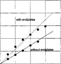
To conclude the consideration of the jet-flapped wing in the extreme ground effect, a comparison is presented in Fig. 6.12 of the results of the asymptotic theory with the experimental data of V. P. Shadrin, obtained in a wind tunnel for a rectangular wing with endplates. Note that, when conduct­ing calculations by using the asymptotic theory, account was taken of the jet reaction force and the presence of the endplates. For large magnitudes of the blowing angle, the reactive components of the jet in the vertical and horizontal directions have to be predicted by the formulas

It is worthwhile to mention that in the experiments conducted by Shadrin a model of a rectangular wing of aspect ratio Л = 1 with a “Gottingen” type foil section with an almost flat lower surface was tested. The relative thickness of the foil was equal to 11%, and the width of the jet injection slot with respect to the chord was 0.0053. Specially designed changeable trailing edge elements provided variation of the angle of blowing r, measured with respect to the flat lower surface of the wing. The injection of air was provided by special fans built into the model.

Consider a jet-flapped foil with the upper and lower surfaces described by yu and y moving above the flat ground at incidence в. The jet deflection angle is designated r, and the jet momentum coefficient Cy In the simplest case of the extreme ground effect, that is to the lowest order, we have to solve a simple differential equation

Equation (6.85) has to be solved with the following trailing edge condition:

(6.86)

Solution of the flow problem in an approximation of the extreme ground effect is straightforward. The lift coefficient was obtained in the form

СУі = l-(l-«j)2(l-Cyo), (6.87)

In the concrete case of a flat plate of infinite aspect ratio with a jet flap in the extreme ground effect, expression (6.88) yields

(l-*j)2 . (1 -ТуїЩЩ1

1+9 1+9

where 6 = 6/h and h is the relative ground clearance. The general algorithm of the flow problem solution enables us to proceed to higher approximations. Omitting intermediate calculations, one can present the following formulas for the lift coefficient of a moderately thick foil with a jet flap:3

– {Б2 – A2 + (0 + ^) (r^ + in

-(l-«j)[51-y1′(0)(l-«j) + y((0)(l-lnTr)] Ґ^-Л (6.93)

Jo У x))

(Vw ~ V2O1 + y/y~)

(Vvi + vIO1 – VS5D ’

For «j = 0, these formulas for Cy yield corresponding formulas for the foil without a jet flap, obtained in paragraph 4.1. In the case of a jet-flapped flat plate in the extreme ground effect, when yu = y = 1 + Qx,

That is, with thickness of the order of the ground clearance.

– j)

Figure 6.9 presents the lift coefficient Cy of a flat plate versus the angle of pitch 9° for different magnitudes of the momentum coefficient Cj and the angle of blowing r° = 30° for h = 0.1.

Figure 6.10 shows the dependence of the lift coefficient of a jet-flapped plate upon the relative ground clearance for r° = 15°, 9° = 2° for different magnitudes of the jet momentum coefficient Cy Linearizing the expression for the lift coefficient Cy of the flat plate, we obtain the formula

where 7e = 0.5772 is Euler’s constant. This formula is identical to the ex­pression derived within assumptions of the linear theory in Kida and Miyai [50].

From the viewpoint of use in the transitional modes of motion (takeoff and touchdown) the so-called jet flaps have a certain practical interest. These flaps are formed by high-speed jets, utilizing the reserve of the air exhaust of turbojet engines blown through narrow slots of the trailing edges of the lifting system. Whereas the increment of lift due to the deflection of rigid flap is always accompanied by a certain increase of drag, jet flaps do not have this deficiency because the major part of the jet momentum gives rise to the thrust. Consequently, jet flaps favorably combine propulsive and lifting properties. One should also point out another reason that justifies the use of jet flaps. When the vehicle is operating in transient modes above rough seas, rigid flaps can touch the sea surface, thereby experiencing considerable hy­drodynamic loads. The latter circumstance can lead to failures in operation of the flaps and the corresponding flap control systems. The use of nonrigid devices, based on jet blowing, gives the possibility of controlling the lifting properties of the lifting system, including the cases when the jets touch the water surface. Assuming that the relative ground clearance is small the prob­lem of determining the aerodynamic characteristics of a wing with a jet flap can be effectively solved by the method of matched asymptotic expansions.

We start with the formulation of a nonlinear flow problem for a jet-flapped wing in the ground effect.

We consider a wing in steady motion with a jet flap along the trailing edge; see Fig. 6.8a.

In what follows, it is assumed that the jet is vanishingly thin. The latter assumption was introduced for the first time by Spence [143], who studied the two-dimensional problem for the flow past a foil with a jet flap in an unbounded fluid. No account was taken in Spence [143] of the ejection effect of the jet upon the surrounding fluid. However, both the results of Spence and other works, see, for example, Maskell and Spence [144], utilizing the

FLOW SUBDIVISION NEAR THE JET FLAP

b.

Fig. 6.8. Scheme of the flow past a wing with a jet flap in the ground effect: (a) general view; (b) near the jet flap.

hypothesis of the thinness of the jet, are in fair agreement with the experi­mental data even for large deflection angles up to 60°. These considerations justify the validity of the adopted mathematical model of a thin jet, in which expansion of the jet due to involvement into the motion of particles of the surrounding fluid is neglected.

The velocity potential of the flow past a wing with a jet flap should satisfy the Laplace equation, the flow tangency conditions on the wing and the jet sheet, the condition of the decay of perturbations at infinity, and the dynamic condition upon the jet surface. The Kutta-Zhukovsky condition at the trailing edge should be replaced with the requirement that the jet is blown at a given angle to the chord of the wing.

As in the general algorithm of the solution of the flow problem discussed in section 2, the flow field is conditionally subdivided into characteristic regions: the channel flow V under the wing and the jet sheet; the upper flow, including the region Vu above the wing; the jet sheet and part of the ground outside of the “shadow” of the wing and the jet on the ground; the regions of local flows near the leading and side edges Ve; and the local flow region in the vicinity of the trailing edge with a jet flap Dj. Below, based on the assumption of
the smallness of the relative ground clearance h <C 1, the main stages of the asymptotic solution of a steady flow problem for a wing with a jet flap will be shown. In accordance with the general hypothesis, the deflections of the jet sheet from the plane у = h are assumed to be comparable to the ground clearance, that is,

h-y} = 0(h). (6.38)

As indicated in section 2, such an assumption enables us to account for non­linear effects, at least in channel flow, with an asymptotic error of О(h2).

Special consideration is required of the local flow near the trailing edge with a jet flap. As for the rest, the solution procedure does not differ signifi­cantly from the approach discussed in section 2 for a wing without a jet flap. Therefore, corresponding modifications of the velocity potentials in regions Di, Vu, and Ve will be discussed very briefly.

At first, consideration is restricted to a vanishingly thin flat wing with a straight trailing edge moving at zero incidence. The full problem for the perturbed velocity potential <p is described by the Laplace equation

dx-2 dy2 dz2 ’

and the following boundary conditions:

• Flow tangency conditions on the wing, ground plane and the jet sheet:

• Dynamic condition on the jet:

Interacting with the oncoming stream, the jet experiences deformations. As a consequence, centrifugal forces occur proportional to the local lon­gitudinal curvature. These forces are balanced by the pressure difference across the jet surface

p – p+=/CC’/x, (x, z)eSj, x < 0, (6.43)

where the pressure can be calculated by the formula

JC is the curvature defined though the coordinates y} of the jet surface as

C^C^(z) = 2l(z)/pU^l is the sectional coefficient of the jet momentum, 1(2) is the sectional jet momentum, plus and minus correspond to the upper and lower surfaces of the jet sheet, and Sj is the area of the jet sheet. The total jet momentum coefficient can be calculated by the formula

(6.45)

square of the root chord.

Rewriting the dynamic condition (6.43) taking into account (6.44) with asymptotic error 0(/i2), we obtain

In what follows, it will be shown, that for small relative ground clearances h, the main modification of the jet surface takes place in the downstream

loses longitudinal curvature, the pressure difference across it vanishes, and (in the case of a finite aspect ratio of the wing) generation of a vortex sheet begins. It can be easily seen that the dynamic and kinematic conditions work automatically in the case of a vortex sheet.

• The requirement of a jet blowing at a given angle r with respect to the chord of the wing:

As noted before in the problem under consideration, the Kutta-Zhukovsky condition at the trailing edge is replaced by the requirement that the jet should be blown at a given angle r = r(z) with respect to the chord at cross section z = const., i. e.,

душ

arctan —^ = r(z). for x = 0,

ox

where Xj is a local x coordinate, directed upstream.

• The condition of the decay of perturbations at infinity:

V(p —> 0, x2 + y2 + z2 —> 00.

Now, we turn to the asymptotic solution of the local problem of flow near a trailing edge with a jet flap. Consider a local flow in close proximity to a trailing edge equipped with a jet flap. Introduce local coordi­nates stretched in vertical and longitudinal directions, i. e.,

‘j а^( 0,г)]’ Vi a2{h*(0,Z)]

where /i*(0,z) is the local distance of a point on the trailing edge from the ground at a given cross section z = const., in our case of a wing of zero lateral curvature one can set h*(0, z) = h.

The stretching functions o and cr2 are to be determined by the least degeneracy principle. Note that, depending on the choice of the stretching functions and the lowest order asymptotics of the local flow potential in the region Dj, it is possible to distinguish different local subdomains for which the local flow descriptions would have corresponding distinct limiting forms. The subdivision of the jet flow domain Vj into different subdomains, as well as respective orders of coordinates, are shown in Fig. 6.8.

In the subdomain V^, independent variables are of the order Xj = 0(h) and 2/j = 0(h), so that one can set o(h) = h and 02(h) = h. Substitution of stretched variables in the full flow problem leads to the local flow problem in the immediate vicinity of the hinge of the jet flap. The solution of the latter problem was obtained in the following form:

• On the upper surface of the wing-jet,

g£ = _^in%+K+ (6’48)

• On the upper surface of the wing-jet,

= ~~ ln[l ~ ехрСтпг,,] + K7, (6.49)

where <p-}1 is the flow velocity potential in subdomain 2?^, — x^/h, 7£r,

and Tfcjj are unknown parameters to be determined by matching.

It follows from expressions (6.48) and (6.49) that the flow velocity near the point of blowing has a logarithmic singularity with different signs on the upper (acceleration) and lower (deccelaration) surfaces of the wing-jet. In subdomain X>j1? the jet degenerates into a segment of a straight line, so that the kinematic boundary condition coincides with the requirement that the jet is blown at a certain angle. The solution obtained in is two-dimensional and describes the local flow at distances of the order of 0(h) from the hinge of the jet flap. The most complete description of the jet can be obtained in subdomain V]2. Under the wing and jet c Pj2, it is convenient to choose the stretching function in the vertical direction as 02(h) = h. Longitudinal stretching о і (h) should be selected so that the mathematical description of the jet is the least degenerate. It means that to the lowest order, one has to retain both the dynamic and kinematic boundary conditions on the jet. We analyze in more detail the procedure of constructing the solution in subdomain V]2. To retain the channel flow for h —> 0, it is logical to assume later on that for h -> 0

o2 = h<£o1(h). (6.50)

Equation (6.50) implies that in the limit /1 0, we will obtain a one­

dimensional description of the flow under the wing and jet in the vicinity
of the flap. In this case, the dynamic boundary condition on the jet acquires the form

(6.51)

The governing Laplace equation, it can be shown as previously, reduces to

The distinct limit for the system (6.51) and (6.52) is secured by the following choice of the stretching function (J{h) and the lowest order asymptotics of the local flow potential:

~ Gi(h)(p-} and <Ji(h) = y/h. (6.53)

With this in mind, equations (6.51) and (6.52) can be rewritten as

To obtain an equation describing the configuration of the jet sheet, we first integrate (6.55). We determine the constant of integration by requiring that at downstream infinity (x^ —> — oo), the jet becomes horizontal at any given cross section z = const. Therewith f/j -» y-}oo(z), and the perturbation ve­locity in the channel flow between the jet and the ground vanishes, i. e., for

where y-}oo(z) has to be determined by matching. Therefore,

Using (6.57) to exclude d(f-Jdx-n from (6.55), we derive the following differ­ential equation for determining the jet configuration:

C. wgf = 1 – fr – («8)

Multiplying both parts of (6.58) by yj, we can rewrite this equation as

Consistent with the previous requirement that for щ = щ{Щі) for any given z = const, the jet becomes horizontal, its slope must vanish too, i. e., for

X -» —00

Щ

dx^

Hence, we can determine the constant

C* = –

Thus, the differential equation governing the form of the jet becomes

It is not difficult to integrate (6.63) to obtain the following implicit equation for yj = Уі(хк):

Now, we can apply the requirement that the air should be blown from the trailing edge at a prescribed angle r = r(,z). Using (6.46) and accounting for the order of magnitude of the jet coordinates, that is,

Ф)

Vh,

and the distance of the jet from the ground far downstream is

Уіос (z) = 1 – Ф) Ш (6-70)

Setting y-}oo = 0 in (6.70), we can determine for which combination of sectional magnitudes of the parameters CM, r, and h the jet would touch the ground at a given cross section z = const.:

For a uniform spanwise distribution of the jet deflection angle, the ground clearance and the jet momentum coefficient, equation (6.71) can be inter­preted as a condition of blockage, i. e., the situation when the jet touches the ground everywhere spanwise

and the blockage occurs at a distance

from the trailing edge.

The longitudinal velocity in a narrow channel under the jet sheet is given by equation (6.57), where y-]oo is described by (6.70). The spanwise distri­bution of the longitudinal perturbation velocity at the trailing edge can be obtained by setting Xj = 0,yj = 1, wherefrom

Due to the conservation of mass, the magnitude of dip-Jdx^ is practically the same as the perturbation velocity under the wing in the vicinity of the trailing edge. Therefore, to the lowest order, the boundary condition for the

channel flow equation at a trailing edge equipped with a jet flap can be written identically as

a-t(o’z)=T{z)fW – (6’76>

This can also be shown through the matching process.

The flow potential in the upper part of subdomain V]2 (x$2) was found in the form _

Vh = hvt + Лл/л(г/^- + V? ih) +0(h2), (6.77)

where (p+ and cpf (xj2) are unknown functions to be determined by matching. The next characteristic subdomain of the flow near the jet flap is Dj3, which is located above the wing and jet; see Fig. 6.8. In this subdomain, y} = О(Vh) and Xj = О(y/h). The expression for the flow potential in 2?j3 was found in the form

^ J 9i(0 Ц(Чз – О2 + У*,] d£+ • • •. (6-78)

where g(h) is an unknown gauge function of h, q(£) is an unknown function, and xj3 = xj2 = X) jyjh. Thus, as a result of the asymptotic analysis of

the flow field in near the point of jet blowing, we can determine the

characteristics of the flow in subdomains Dj1? Dj2, and V]3 with the help of expressions (6.57), (6.77), and (6.78). The unknown parameters and functions are determined by matching.

Continuing the discussion of particular features of the asymptotic algorithm for a wing with a jet flap in the ground effect, some cor­rections will be shown briefly, which have to be introduced into a general algorithm of the solution in the particular case of a wing with a jet flap. In the upper flow region Du, the expression for the potential (pu (2.31) has to be supplemented by the term

~ [ – cU, r = ^(x-02 + y2 + (Z – 02, (6-79)

47Г J2 r

which represents the potential of the distribution of sinks with strength along the trailing edge І2 and models the influence of the jet flap upon the upper flow. In subregion Ve near the leading edge and side edges, the velocity potential is given by expression (2.39), in which the coefficients a* depend on characteristics of blowing. If the wing has endplates, their influence upon the aerodynamics of the lifting system can be determined in the same fashion as for a wing without a jet flap.

In the channel flow V the equation for determining the potential (f has the same form as that for a wing without a jet flap. For zero pitch angle, the equation for the lower flow potential is
with boundary conditions at the leading edge and side edges to be determined by matching. Below, without going into details, some results are presented of the matching needed for further calculations. Matching the upper flow potential <pU) valid in region T>u, with solutions ip^ and ^ in subdomains Vi2 and Vj3 enables us to find the quantities g(h), j, and

where describes ordinates of the jet for large Xj2 —> —oo. Note that Уіоо depends on z, i. e., varies along the span, and Qj(z) is negative, i. e., represents the productivity of sinks, modelling local effects in the upper flow subdomain, connected with deformation of the jet surface from the trailing edge downstream.

5.1 An Estimate of the Influence of Endplates

A definite pecularity of the wing-in-ground-effect vehicle compared to the airplane consists of the presence of endplates. Endplates are mounted at the wing’s tips and are intended to decrease leakage of air from under the lifting system. Consequenly, the mounting of endplates results in the augmentation of lift or in a decrease of the induced drag for a given lift. In practice, the configuration of the endplates can vary. Figure 6.1 illustrates schematically some of the possibilities.

According to the approach adopted herein, to account for the influence of the endplates upon the flow past a wing in the ground effect, one has to solve the corresponding local flow problem in the vicinity of the order of 0(h) of the tip of a wing equipped with an endplate. Strictly speaking, the local flow solution includes both homogeneous and nonhomogeneous parts, as is the case for a wing without endplates. However, it can be shown that the ratio of the nonhomogeneous to the homogeneous component is of the order of 0(h). Therefore, to the leading order, the analysis can be restricted to constructing only a homogeneous (circulatory) component of the flow around the wing tip of a given geometry. Such a solution will be reduced to the conformal mapping of the local flow domain onto the interior of the unit strip 0 < S/ae = t/>ae < 1 in the plane of the complex velocity potential /ae = (fae + i^ae-

The solution procedure for the problem will be illustrated for the flow past a rectangular wing with vanishingly thin endplates.

b

K. V. Rozhdestvensky, Aerodynamics of a Lifting System in Extreme Ground Effect © Springer-Verlag Berlin Heidelberg 2000

At first, consider the local flow problem for an edge with a thin lower endplate of height hep. Introduce a complex variable ( = v+y in the physical plane. Map the domain of flow in the £-plane onto the upper half plane ^sg = 92 > 0 by the Christoffel-Schwartz transformation; see e. g. Lavrient’ev and Shabat [129]. The point-to-point correspondence for the conformal mapping is shown in Fig. 6.2. The mapping is obtained in the form

> __ і (t + l)(7ep t) 2(1 7eP)£

7Г (l-t)(t + 7eP) 7eP7r(l-t2)’

where

The parameter 7ep is related to the height of the endplate through the following equation:

where h* is the local ground clearance, i. e., the distance from the wing’s surface to the ground near the endplate. The mapping of the upper half plane > 0 upon the interior of the unit strip 0 < ^fae < 1 of the plane of the complex potential is performed by the function

g = 9l + i#2 = ехр(тг/ае). (6.3)

For points on the wing,

• on the upper surface,

C = £ + i, 9 = 9l < -P, /ae = ty^ae + i, ty^ae > 0; (6.4)

• on the lower surface,

C = £ + i, 0 >g = gi> – P’, /ae = y? ae + i, </>ae < 0. (6.5)

At the points on the endplate for v — 0,

• on the exterior surface of the endplate,

C = iy, о > у > = – hep, —/3 < gi < —1,

/ae V^ae “b / V^ae ^ (6.6)

• on interior surface of the endplate,

C = іУі = ~hep ^2/^0, —1 < <7i < —(3 ;

/ae — V^ae + І, V^ae ^ 0[28]

To match the local flow solution for the endplate with the asymptotic descriptions of the upper flow and channel flow, we need to know the far – field behavior of the edge flow potential at?/ —> — oo, у = 1 ± 0. These estimates are readily obtained in the following form:

Far from the endplate on the upper surface of the wing (z> —> — oo, у =

1+0),

V? ae ^ – ln(7ep7TZ>). 7Г

The general form of the solution valid near the wing tip with an endplate has the following asymptotics:

(fe = hai(pae + /га4 + О (/г2). (6.10)

Recalling that the upper flow potential in the immediate vicinity of the wing’s edge has the following asymptotic behavior,

<Aii – ln(h*9) + – A2 + 0(h2), (6.11)

Z7T 7Г

and matching (6.11) with the asymptotic representation of (6.10) far from the edge, one obtains taking into account (6.9),

Thus, in the problem under consideration, the channel flow potential can be found, as previously, by solving the quasi-harmonic equation (2.22) for the nonlinear case and the Poisson equation (3.14) in the linearized case. However, here, the boundary conditions to be applied at the wing’s planform contour, incorporate the influence of the endplates. Note that in the linear case, the local clearance of the wing near the endplate should be substituted by h.

A relatively simple solution can be derived for a rectangular wing of a small aspect ratio Л; see Rozhdestvensky [44]. In this problem, the upper flow potential outside of the tips is constructed in the same way as for the small-aspect-ratio wing without endplates. The channel flow is determined by using the equation (3.48) with boundary conditions

where h — h/X. The lift coefficient for the lower endplates was obtained in the form

where h — h/X and parameter 7ep is linked to the endplate height hep by equation (6.2). For hep —> 0, the lift coefficient becomes equal to that for the small-aspect-ratio wing without endplates, i. e.,

In Fig. 6.3, some calculated results are compared with experimental data for X = 1, h — h — 0.057, hep/h = 0.875.

1.0

0.0

The augmentation of the lift coefficient of the wing resulting from the installation of endplates can be characterized by the coefficient

Some calculated curves, showing the behavior of this coefficient versus the relative height hep of the endplate for different clearances h of the wing-in­ground effect are presented in Fig. 6.4. It can be observed from Fig. 6.4 that the utilization of endplates may result in a considerable increase in the lift. In other terms, for a wing with endplates, the effective aspect ratio may quite noticeably exceed the geometrical aspect ratio.

We turn to the consideration of endplates of a more complex configuration; see Fig. 6.1b. Suppose that the upper part of the endplate has a height hep, whereas the lower part has the height /12. The local flow velocity potential can be obtained by the same technique as for the simpler lower endplate. The lift coefficient for the wing of small aspect ratio with endplates under consideration was found in the form

where parameters 71 >72 > l//?7 are related to the dimensions of the end­plate by the following relationships:

Some results illustrating the influence of the lower and upper parts of the endplate upon the lift coefficient of the wing are presented in Fig. 6.5. It is easy to see from the analysis of the graph that the upper parts of the endplates have an insignificant effect upon the increase of the lift. The same conclusion was drawn by Ermolenko et al. [133].

Now, return to a more general problem of the influence of endplates upon the aerodynamics of a wing of arbitrary aspect ratio. As shown above, when the wing tips are equipped with endplates, a change occurs in the bound­ary conditions, starting from an approximation of the order of 0(h). Conse­quently, functions ipx and <p2, which characterize, respectively, the first and the second approximations for the channel flow potential, are not dependent upon the parameters of the endplates. On the other hand, the influence of channel flow upon the upper flow is defined by the strength Qi of the source (sink) singularities, distributed along the wing’s planform boundary contour. Due to the fact that

within the approximation considered, the endplates practically do not affect the upper flow.

The previously mentioned considerations lead to the following conclusion: to account for the variation of flow past a wing in the ground effect due to the presence of endplates, it is sufficient to solve the problem just for the corresponding increment of the channel flow potential.

The corresponding boundary problem with respect to this increment (pep for unsteady linearized1 flow around a lifting surface with endplates can be written as follows:

where for thin lower endplates the function G is given by

G(7ep) = + In (1^7ep)3-, (6.29)

1 7ep °7ep

Nonlinear version can be handled in a similar fashion.

and parameter 7ep is related, as earlier, to the height of the endplate by equation (6.2). Having at our disposal the lowest order flow problem solution, we can readily obtain information on the influence of the endplates for both the steady and unsteady motions of a wing near the ground.

Consider, as an example, the steady motion of a flat rectangular wing with lower thin vertical endplates at given angle of pitch в. The relative increment of the lift due to the endplates is found in the form

к>е p — = 1 + /іС?(7еР)Л(Л) + 0(/i2), (6.30)

Су

where Л is a function of the aspect ratio

= 4 E”0(-l)ntanh2(gnA2/4)/g3

7гЛ2 E~=otanh<2ntanh(W2)/9n ’

Some calculated results for the coefficient кер versus the aspect ratio Л and for different hep/h are presented in Fig. 6.6. In the limiting cases of large and small aspect ratios of the wing and for hep < 0.5/г, the expression for nep is simplified:

• For Л —> 0,

It is not difficult to verify that with an asymptotic error О(h) (where h = h/X) the first of these formulas is compatible with expression (6.18), which was derived from a straightforward solution of the flow problem for a small – aspect-ratio wing.

It follows from the analysis of the formulas presented and Fig. 6.4 and 6.6 that, for a wing near the ground, the efficiency of endplates increases with a decrease in the aspect ratio and/or a decrease in the gap between the lower tip of the endplate and the ground.

In the case considered before, the endplates were assumed to be vanish­ingly thin. Inclined and/or thick endplates can be handled in a similar fashion. Consider an endplate of a more general polygonal configuration (Fig. 6.7). We map the flow domain around the endplate onto an upper half plane Э > 0 by the Christoffel-Schwartz transformation so that the point As corresponds to аз — —1 (the point-to-point correspondence is shown in Fig. 6.7). The mapping function is

where

F(g) = {g – a2r~g +1)“3-1 • • • (g (6.35)

where a. k = OLk/7Г are the external angles of the polygon.

The Christoffel-Schwartz constants аг, а±,…, dk~ 1 are determined taking into account the point-to-point correspondence in the planes £ and g and depend on the parameters that characterize the geometry of the endplate. The

lift coefficient for a small-aspect-ratio wing-in-ground effect with endplates of polygonal cross section was obtained in the form

The endplate configurations presented in Fig. 6.1a, b,c, d can be derived as particular cases from the polygonal shape considered.

Consider a moderately curved foil in a two-dimensional steady compressible flow near a flat ground. To the lowest order, the corresponding channel flow equation, formulated with respect to the relative motion velocity potential фх, can be derived from the more general three-dimensional equations (5.14)- (5.16) in the form

1 + ^(7 – 1)M,2(1 – w2) – ^s(*)M02u-jlu2 = 0,

Grouping with respect to d In ys and dp,

(1 + pp){ 1 – p) dlnys – 1(1 + pp)dp + 1m02(1 – p)dp = 0,

Integrating (5.58),

In2/s = ~^ln(l – p)~ ^^-hi(l +pp)+]nC*. (5.59)

Applying the trailing edge condition ys(0) = l, p = 0, we find that С* = 1 so that

4 = (X ~pX1 + PP)M°/>1- (5-60)

Vs

We introduce the pressure coefficient

ys(x) = l + 9x, y’s = e re Є [-1,1],

so that the lift coefficient is given by

(5.63)

Some calculated results, corresponding to the case of a flat plate, are pre­sented versus the relative pitch angle 9 for the Mach numbers M0 = 0.5 and M0 = 0 (incompressible flow case) in Fig. 5.10.

In paragraphs 5.1. and 5.2., both nonlinear and linear compressible flows around a wing in the extreme ground effect were discussed, and corresponding approximate mathematical models were proposed. In this paragraph based on a linear formulation, the flow problem for a rectangular wing in the extreme ground effect will be treated for harmonic dependence of perturbations on time. Recall equation (5.19) for linear compressible flow past a wing in the extreme ground effect, omitting subscript ul{K.

With the intention of investigating a representative example of heave oscil­lations of a rectangular wing, we represent the instantaneous local gap and velocity potential as

/i*(x, 2, t) — h — h0iexp(ikt), (p(x, 2, і) = ф(х, z) exp(ifc£), (5.35)

where к = ujC0/U0 is the Strouhal number, і = /—Ї – Taking into account of (5.35) equation (5.34), yields

h0k

T

We express the complex amplitude of the channel flow velocity potential ф in terms of a series that satisfies the condition of zero loading at the tips of the wing:

°° 7Г

<p(x, z) = ^Txn(x) cosqz, qn = -(2n + l), (5.37)

n=0

The resulting equation with respect to functions Xn(x) can be written as (1 – M02)X" + 2iMg k2X’ + (k2M^ – qn)X = Q, д = _4^(~1)" (5 39)

The characteristic equation for (5.39) is

к

with roots

(5.41)

(5.42)

where Xnp&rt(x) is a particular solution equal in this case to Q/(k2M{2 — q2).

Recalling that the perturbed flow potential to this order should satisfy two boundary conditions, namely, ip = 0 at the leading edge (x = 1) and

=0

dx dt

at the trailing edge (x = 0), we can write, respectively,

Ф( 1) =0, Xn( 1) = 0 (5.43)

and

g-i^ = 0, X’n-ikXn = 0 x = 0, (5.44)

Applying the requirements (5.43) and (5.44), we can obtain the following expressions for the coefficients of the solution series

A _ V A* = X ______________________ ifcexp(/i2n) + !Hn – ik______________

П npart „ – p-exp^^^-i^-exp^)^-^)’

ifcexp(/Ui„) + Ціп – і к

"part^n – «part exp(p2n)(Atln “ І&) ~ ЄХ-Р(Ціп)(М2п – Ік) The lift coefficient is obtained by integrating the loading

The final expression for the complex amplitude of the lift coefficient is

Cy(t) = C$h + tfh, (5.49)

where

rh _ Щ, rh=*£v

y~ h0k’ V h0k2’

where 5ft and 5 are real and imaginary parts of the expressions.

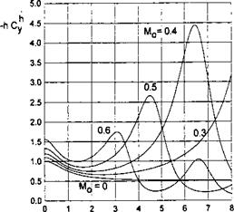
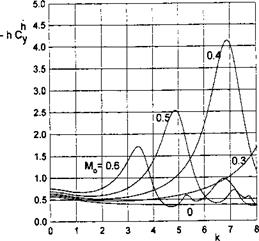
Some results for heave derivatives of the lift coefficient, multiplied by the steady state ground clearance, i. e., hCy and hCy are presented in Figs. 5.2­5.7 versus the Strouhal number and for different Mach numbers for a rect­angular wing of aspect ratio A = 1,2,3, oo. The characteristic feature of the curves of (—hCy) as a function of the Strouhal number consists of the oc-

A = 2.

currence of pronounced maxima that tend to decrease and shift to smaller Strouhal numbers with increases in the Mach number and the aspect ratio.

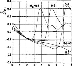
The analysis of the curves representing hCy versus the Strouhal number shows that for the range of Strouhal numbers, corresponding to the max­ima of (—hCy), points of “loss of vortex damping” appear, i. e., zeros of the

quantity hCy. These features of the unsteady aerodynamics of a wing in an unsteady compressible ground-effect flow can be interpreted as an “acoustic resonance.” The theoretical possibility of the occurrence of acoustic resonance was discussed by Sohngen and Quick [140] in connection with unsteady gas flows through axial compressors and within a more general formulation of flat plate cascade oscillations in compressible flow by Gorelov et al. [141].

The same conclusions were drawn by Efremov and Unov [142], who studied oscillations of a foil in a two-dimensional flow in the presence of the ground. Acoustic resonance may take place when the frequency of oscillations of a wing in a restricted compressible flow3 coincides with some of the fundamen­tal frequencies of oscillations of compressible flow with the same boundaries.

A linearized version of a steady compressible flow around a wing at arbitrary relative ground clearances is described by the following boundary problem:

^ = at ix’z)^S’ У — h±0; (5.23)

^ = 0 at (x, z) Є 67, у = 0 + 0, (5-24)

where М0 is the Mach number of the oncoming stream. Using the Prandtl – Glauert transformation for the у and z coordinates, у’ = y/l — M2, z’ — z у/1 — M2, x’ = x, we obtain the following problem for an equivalent incompressible flow: • Equation:

d2ip d2ip d2if _ &r’2 + dy’2 + ^’2 “

Note that the original Prandtl-Glauert rule implies that only the x coor­dinate is transformed into x’ = xj — M02. Here we prefer to retain the same chord length. In fact, both transformations lead to identical results. • Boundary conditions

where /?м = /l — Ml As seen from (5.25)—(5.27), in a linearized steady state approach we account for compressibility by utilizing the results obtained previously for incompressible flow, but in a space “squeezed” both vertically and laterally. In particular, we consider an equivalent incompressible flow for a wing of smaller aspect ratio A’ = Л • /?м – In addition, the downwash on the surface of the equivalent wing is 1//?m times larger than in a corresponding compressible flow problem.[25] The aforementioned two factors are the same as in unbounded flow. A distinctive feature of the flow in ground effect is that the equivalent wing moves at a smaller ground clearance hf = h • /?м – To compare the influence of compressibility upon a wing in an unbounded fluid and in the extreme ground effect, we consider the simplest cases of a flat plate of infinite and small aspect ratio. For a two-dimensional incompressible flow the following are the expressions for the lift coefficient:

Turning to the compressible flow case by the of Prandtl-Grauert correction, we can obtain the following formulas for the lift coefficient:

• In an unbounded fluid,

Now, it is easy to see that for a wing of large aspect ratio in both unbounded and bounded flow, there is an increase of the lift coefficient due to compress­ibility. However, in the ground effect, the influence of compressibility is more pronounced. For example, for a Mach number equal to a 0.8, an increase of the lift in the extreme ground effect is almost twofold compared to unbounded flow. It should be noted that Efremov [71], studying a thin foil, also came to the conclusion that, in proximity to the ground, the influence of compressibility leads to a noticeable increase in the lift coefficient. Such a conclusion can be easily interpreted in terms of the Prandtl-Glauert trans­formation, if one accounts for the fact that the equivalent wing flies closer to the ground, hf = hyj — M0[26].

м0

Figure 5.1 features a compressibility correction in the form of the ratio of the lift coefficients in compressible and incompressible flows versus the Mach number for wings of different aspect ratios in the extreme ground effect (Rozhdestvensky [41]). This correction can be shown to hold for a practical range of ground clearances (up to 0.15) with an asymptotic error of the order of 0(/i). For comparison, the curve corresponding to the unbounded two­dimensional flow compressibility correction factor /?м = Л — M0[27], is plotted in the same figure (dashed line).

Now, we can proceed to the case of the small aspect ratio, for which in incompressible flow

• In unbounded flow, as predicted by the Jones theory,

Су — 2 a%

In the extreme ground effect, see formula (3.69),2

r – —

y 6h ‘

Using the Prandtl-Glauert correction, i. e., replacing respectively Л, h, and a by A’ = /?мА, Ы — and о! — а//?м> we obtain a result, which

reads similarly for both unbounded and bounded flow, namely, for wings of a small aspect ratio, the influence of compressibility upon the lift coefficient becomes negligible.

In three-dimensional, compressible, isentropic flow, the following relation­ships can be shown to hold (see Ashley and Landahl [161]):

• Equation of fluid motion

where ф is the velocity potential of relative fluid motion related to the per­turbed velocity potential cp through the equation

ф = – x + (p,

as and aSo are, respectively, the local velocity of sound and the velocity of sound at upstream infinity, M0 = U0/aSo is the Mach number in the unper­turbed oncoming flow, and 7 is the ratio of the specific heat of gas (isentropic parameter); for air, 7 = 1.4;

Excluding (as/aSo)2 from (5.1), we can derive the following equation to de­termine the relative velocity potential:

_M°2 Ш + !(w)2 + ‘ V(W)21= °- (5-4)

In the channel flow region D, we introduce stretching of the vertical coordi­nate у — у jh and seek ф in the form of an asymptotic expansion

(5.5)

where

{ФІ, ФГ) = 0(1), Фї = фн + Ь1п^фІ2 + 1гф1з. (5.6)

Passing over to the channel flow variables and accounting for the adopted asymptotics (5.5) of the potential in the gap between the lifting surface and the ground, we obtain the following relationships with respect to the potential function ф*:

where Л/і,2 are nonlinear differential operators in the two variables x and г:

Integrating (5.10) once with respect to у and using the flow tangency condi­tions for ф** identical to (2.15) and (2.17), where </?** — x should be replaced by </>**, we obtain the following channel flow equation for compressible isen- tropic flow (Rozhdestvensky [41]):

h* = h*/h, /г* = h*(x, z,t) is a prescribed instantaneous gap distribution. To solve the lowest order problem (the extreme ground effect), one has to replace ф* by фг and apply the following boundary conditions at the planform contour:

(fx = x + фг =0 at the leading edge, (5.15)

рг = 0 at the trailing edge. (5.16)

Inspecting the expression for the pressure coefficient in compressible flow, (see Ashley and Landahl [161]),

To satisfy (5.16) for compressible case, it is sufficient to require that

For small perturbations, linearization of equation (5.14) leads to the following lowest order problem with respect to the perturbed velocity potential :

<9×2 <9z2

• Boundary conditions at the planform contour:

(рг =0 at the leading edge, (5.20)

Ph — 2 f-гг1 – =0 at the trailing edge. (5.21)

ox ot )

It is practical to extend the analysis of the aerodynamics of a wing in the ground effect to account for the dynamic compressibility of the air. In fact, the cruise speed of ground-effect vehicles can amount to half or more of the speed of sound. At the same time, it is known that the problem of unsteady subsonic flow is one of the most challenging in lifting surface theory; see Belotserkovsky et al. [139]. The complexity of the problem partly stems from the fact that in a compressible fluid the perturbations propagate with finite speeds.

The problem of compressible flow past a wing in the extreme ground effect can be treated on the basis of the approach, similarly to that applied in section 2 for an incompressible fluid. Here one adopts the same assumption as previously, stating that both deviations and slopes of the surfaces of the wing, vortex wake, and the ground should be small, i. e., of the order of the relative ground clearance; see (2.1). In this case, it becomes possible to linearize the flows above the wing and the wake and introduce linearizing simplifications into formulations for edge flows. As earlier, with an asymptotic error of the order of О (h-o), channel flow can be shown to retain almost a two-dimensional nature and incorporate nonlinearity. In what follows, the derivation of the solution will be confined to the leading order of 0(1) and the case of constant speed U(t) = 1. Then, some examples are considered, including linearized steady and unsteady compressible flows past a rectangular wing and the nonlinear flow problem for a two-dimensional foil in the extreme ground effect.

To analyze the linear dynamics of a lifting configuration in the ground ef­fect one needs derivatives of the aerodynamic coefficients with respect to the relative ground clearance h, the pitch angle 0, and their rates h and 6. To determine these derivatives, we consider small unsteady perturbations of a
nonlinear steady-state flow. Such a perturbation analysis enables us to re­tain the nonlinear dependence of the aerodynamic derivatives upon basic steady-state parameters, e. g., adjusted pitch angle, relative ground clearance in cruise, etc. As an example of an application of such an approach, take the case of a rectangular wing with endplates at h -» 0. For simplicity, consider full opening of the flap at the trailing edge, that is, 5{ = 1. Represent the velocity potential of the relative motion, the local ground clearance distribu­tion, and the gap under the endplates in the following way:[23]

Ф(х, і) = фа(х) + <j>(x, t), h*(x, t) = hs(x) + h(x, t),

5ep(x, t) = Sep(x) + h(x, t),

where subscript “s” designates steady-state parameters, whereas the second term in each equation represents unsteady contributions.

Substituting the perturbed quantities in (4.53) and accounting for the description of the steady-state flow problem,

we obtain the following equations for the unsteady flow potential ф(х, і):

When deriving the trailing edge condition for unsteady flow potential in (4.118), it was taken into account that d<j>s/dx = — 1 at x = 0. Using the steady flow equation, we obtain an alternative equation for the perturbed unsteady velocity potential:

Having fulfilled the linearization of unsteady flow with respect to non­linear steady flow, we can consider separately two practical cases of height perturbation and pitch perturbation.

Unsteady Height Perturbation. In the case of height perturbation, h(x, t) = h(t). The perturbation potential can be represented as

ф(х, і) = 4>h(x) h(t) + 4>h(x) h(t).

Assume that the gap under the tips of the endplates in cruise is constant chordwise 5ер(я) = 5ep = const. Corresponding equations for the components of the perturbed solution can be derived in the form

Imposing conditions at the leading edges, we arrive at the following boundary conditions at x = 1 for equations (4.121) and (4.122):

Assuming an oscillatory character of perturbations,9 we relate heave accel­eration and heave displacement, namely, h = —k2h, where к = ujC0/U0 is the Strouhal number based on the chord of the wing. Therewith, we obtain the following boundary condition for the derivatives of the unsteady velocity

potential with respect to h and h at the trailing edge:

Integrating equations (4.121) and (4.122) and accounting for the boundary conditions (4.123) at the leading edge gives the following expressions for the corresponding perturbation velocities and potentials:

To determine the constants c and C2, we apply the boundary conditions (4.124) at the trailing edge. This gives

a + k2 [3 7 (5-а 7

1 + k2 72 ’ 2 1 + k2 72 ’

where

In these expressions, h is the relative ground clearance measured from the trailing edge, Sep = 5ep/h = 0(1), hs(x) = hs(x)/h = 0(1), and vs(x) = d(j)s/dx is the span-averaged channel flow velocity.

The derivatives of the unsteady pressure coefficient with respect to h and h can be derived in the form

It can be seen from equations (4.126)-(4.129) that the derivatives ph(x) and

ph(x) are inversely proportional to the relative ground clearance in cruise,

i. e., are of the order of 0(1 /h).

Unsteady Pitch Perturbation. In the case of pitch motions around the center of gravity h(x, t) = 0(t)(x — xcg), the perturbation potential of un­steady flow can be represented as

ф(х, г)=ф50 + фё0. (4.130)

The derivatives of the unsteady perturbed velocity potential with respect to perturbation in the pitch в and the rate of pitch 6 are governed by the following equations:

The boundary conditions at the leading and trailing edges for equations (4.131) and (4.132) are

The constants сз and C4 can be calculated by using the boundary conditions at the trailing edge.

The derivatives of the pressure distribution, induced by the unsteady variation of pitch, can be determined by the following expressions:

As in the case of unsteady height perturbations, these derivatives are inversely proportional to the relative ground clearance h in cruise.

Derivatives of lift and moment (around the center of gravity x = xcg) coefficients can be obtained by integrating the derivatives of the correspond­ing pressure distributions:

С0в,§ = (4.138)

Jo

1 – z – ^

(x — xcg) рЬ>М,0(д.) (4.139)

Note that in both unsteady height and pitch perturbations, the derivatives of lift and the moment coefficients with respect to h, /1, 0, and 9 are inversely proportional to the relative ground clearance in cruise.

Now, we turn to determining the drag coefficient Cx and its derivatives with respect to height and pitch perturbations. The drag coefficient can be written as

Cx — CXi + CXf (4.140)

with Cx. and CX{ representing, respectively, induced drag and viscous drag. Later on, it will be assumed that the viscous part of the drag does not vary with small perturbations of ground clearance and pitch angle.

As discussed earlier in this chapter, the induced drag coefficient can be obtained by the formula

CXi=CXp+Cs (4.141)

where CXp is part of the induced drag coefficient due to the longitudinal component of pressure forces, and Cs is a suction force contribution. For flat ground, CXp can be written as

r1 d h[24](x)

CXp(x, t) — h J p(x, t) ^ ■ dx. (4.142)

Substituting h*(x, t) = hs(x) + h(t) + 9(t)(x — xcg) and the perturbation expansion of pressure p(x, t) in (4.143), we obtain the following expressions for the derivatives of CXp in height and pitch:

Ch, h,e, e = h Ґ da._ (4Л43)

p Jo dx

The steady-state pressure contribution to the induced drag is given by

cxp, =h Jo рЛх)А‘dx – (4.144)

We consider the suction force contribution to the induced drag coefficient. According to (4.63), it can be determined as