Category Aerodynamics of a Lifting System in Extreme

To reduce a nonlinear formulation to the linear theory, one has to assume that the deflections of the surfaces of the wing, its vortex wake, and the ground, respectively, from horizontal planes у — h • [8] and у = 0 are small compared to the ground clearance h, i. e.,

|2/u, l,w Щ ^ l/g ^ (3.1)

These assumptions lead to the possibility of imposing boundary conditions for the wing and the wake on the plane у = h and boundary conditions for the ground on the plane у — 0. Note that, upon linearization, the quasi-harmonic equation (2.22) is reduced to the Poisson equation. It is obvious that within the linear theory, the pressure is related to the velocity potential through linear differential operators for both the upper and channel flows.

Uniformly valid asymptotic expansions for the velocity potentials on the upper and lower surfaces of the wing can be determined by using the rule of additive composition (see Van-Dyke [38]) in the form

P+ = ¥>U + (<p? e – ^+eu) + (*>£ – <fteu); (2-102)

<P~ =<P 1 + – v>e) + (<?te – ¥4ei)> (2.103)

where (/’u. We^te.^u^teu.^leP^tel and ‘Pi are Siven> correspondingly, by formulas (2.25), (2.39), (2.58), (2.63), (2.78), (2.68), (2.87), and (2.11).

The aerodynamic coefficients of lift Gy, longitudinal moment mz (around a point with abscissa x0), and lateral moment mx can be calculated by using the formulas

Cy = ±JJs(p–p+)ds = ^JJjjp- – p+) dS, (2.104)

mz = і jj{p–v+){x-x0)dS=^ Jjs(p–p+)(x-x0)dS, (2.105)

m* = i JJJP~ ~P+)zdS = p j jiP~ ~P+)zdS, (2.106)

where S is the reference area of the wing related to its root chord squared; Л and l are the aspect ratio and relative span of the wing; and p~ and are

uniformly valid asymptotic expressions for pressure coefficients on the lower and upper surfaces of the wing, determined by the formulas

where <p~ and (p+ are uniformly valid asymptotic representations of the ve­locity potential on the lower and upper surfaces of the wing, determined with help of formulas (2.102) and (2.103). Analyzing expressions for pressure, it is easy to see that for the upper surface of the wing, the corresponding formula is linearized, whereas for the lower surface a nonlinear formula is used. These representations of pressure are compatible with primary assumptions and asymptotics obtained for the flow velocity potentials. In fact, for small geo­metric and kinematic perturbations the flow above the wing is only slightly perturbed. On the other hand, in the flow beneath the wing, induced pertur­bations can no longer be considered small.

To evaluate the lift-to-drag ratio (aerodynamic fineness) of lifting systems in the ground effect, it is necessary to calculate part of the drag due to normal loads. At the same time, one has to take into account the fact that due to low pressure at the wing’s leading edge, the so-called suction force may occur, directed upstream and reducing the drag.

The induced drag of the wing incorporating the suction force can be determined by investigating the flow far downstream in the Trefftz plane. The induced drag coefficient is given by the formula

where /^(z), aWoo are the spanwise distributions of circulation and downwash in the Trefftz plane, whereas S is the wing’s reference area related to the square of the root chord.

To the leading order, this expression can be represented in the form

h fl/2

Cx, = —§ (ph(z)aWldz. (2.109)

* J1/2

Consideration of expression (2.109) shows that for a fixed lift coefficient the induced drag coefficient is of the order of О(h0) and, in extreme proximity to the ground, diminishes in direct proportion to the relative ground clearance.

Sometimes it is practical to be able to evaluate the suction force contribution to the induced drag. The magnitude of this force is defined by the perturbation velocities near the leading edge. As demonstrated by Be- lotserkovsky and Scripatch [130], the leading edge flow is close to that in two-dimensions in the plane, normal to the leading edge planform contour.

Near the edge, all components of the perturbation velocity can be shown to be finite with the exception of component u„, which is normal to the planform contour and lies in the plane tangent to the lifting surface. If the behavior of uv is described by the relationship

Comment on the Definition of the Leading and Trailing Edges in a Nonlinear Formulation. So far the notions of the leading (side) edge and trailing edges have been dealt with without attention to the questions: Where does the transition lie between these and how can we determine the position of the corresponding transition point? It should be said that such transition points may be fixed a priori by the geometry of the planform, especially if its tips are sharp; see Tuck [53]. Otherwise, when the planform contour is suffi­ciently smooth, the position of the transition point is not known in advance, and its determination becomes part of the flow problem. In the nonlinear case, this transition does not necessarily occur at the wing tips, corresponding to the maximum local span.

Following Newman [54], one can define the transition point as that where both leading edge and trailing edge channel flow boundary conditions are ful­filled simultaneously. To the lowest order of 0(1), it implies that at the point (xt, zt) Є l nl2, where subscript “T” denotes the transition point, both

(2.115) and (2.116) hold simultaneously. Introducing the normal-tangent lo­cal coordinates (v, r) and designating by x the (least) angle between a tan­gent to the wing’s planform contour and x axis, one can rewrite expressions

(2.115) and (2.116) at the transition point, i. e., for (x, z) = as

<pu =

Substituting (2.118) and (2.119) in (2.120), we finally obtain the following equation for the determining the position of the transition point as part of the lowest order problem solution:

If the perturbations are small (linearized problem), the squares of the pertur­bation: velocity components in (2.120) can be neglected, which results in the following equation:

~q)~ sin Xt = 0. (2.122)

Therefrom

sinxT = 0 at the transition point. (2.123)

It is easy to conclude from (2.123) that for a linearized problem and a smooth wing planform contour, the transition points coincide with the tips of the wing.

To determine the unknown constants that enter the asymptotic expansions of the solutions in different parts of the flow and also the boundary conditions at the contour of the two-dimensional domain S for quasi-harmonic equation (2.22) of the channel flow, it is necessary to match these expansions in the overlap regions. From a physical viewpoint, the matching procedure is sim­ilar to accounting for the interaction of different parts of the flow. From a mathematical viewpoint the process of asymptotic matching allows attaining uniqueness of the composite uniformly valid solution of the problem.

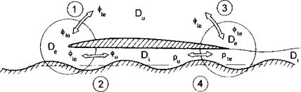
We match of the flow characteristics in the different regions in accor­dance with the scheme shown in Fig. 2.2, where for simplicity the sequence of matching is shown in a two-dimensional case.

• In the first stage, match the velocity potential (pu of the upper flow with the potential (fe of the flow near the leading (side) edge hfa)- This step will result in the determination of parameters аі, а2,аз, а4, and du.

• In the second stage, match the channel flow potential p with potential (fe

of the flow near the leading (side) edge This step gives the possibility

of determining the boundary condition for the channel flow quasi-harmonic equation at contour /1, as well as the magnitudes of d and the strength Q of the contour distribution of sources (sinks) in expression (2.31).

• In the third stage, match the upper flow potential tpu with the trailing edge flow potential (fte – This step will determine parameters 61,6^, 63”, and eu. Imposing the Kutta-Zhukovsky condition in the form of equation (2.5), find the relationship of parameters 6^,63 with parameters b^b^.

• Finally, in the fourth step, match the pressure coefficient in the flow below the trailing edge pe with the channel flow pressure coeffcient p.

In what follows, we use the “asymptotic matching principle,” as introduced by Van-Dyke [38], namely: the “ m-term inner expansion of the n-term outer expansion is equal to the n-term outer expansion of the m-term inner ex­pansion,” where m and n are integers. Note that within the formalism of the method of matched expansions, the term “outer” expansion stands for the asymptotic expansion, obtained in variables, based on the primary charac­teristic lengths of the problem. The “inner ” expansion implies the use of variables stretched with the help of the gauge function of a small parameter so that they have the order of 0(1) in the regions of the nonuniform validity of the outer expansion.

To match in the first stage, it is necessary to derive an asymptotic representation of the upper flow potential pu at points of a normal v in the immediate vicinity of the leading (side) edge. This asymptotic expansion has been obtained previously and is given by expressions (2.25) and (2.32). Replacing the variable v in (2.32) by h*eD, we obtain the following two-term asymptotic expansion:

7Г 7Г

where /г*е, as earlier, is the instantaneous distance of the edge vertex from the ground, which has the order of O(/i0), and (asw) = au(M) — ag(Z,£) is the difference between the downwash upon the upper surface of the wing and that upon the ground in the vicinity of the leading edge. The first term of expression (2.62) is known from the theory of potential functions to reflect the behavior of a potential near a line distribution of sources. Other terms describe the behavior of the surface distribution of sources (simple layer) near the edge. Parameters A(l, t) and A2(l, t) characterize the influence of distant sources. Expressions A and A2 are cumbersome in the general case, so they are not presented here, but will be written for some concrete problems later on.

On the other hand, collecting expressions (2.39), (2.46), and (2.54), we obtain the following asymptotic expansion of the leading edge flow potential far from the edge on the upper surface of the wing (у = 1 + 0):

(file -»ipeu ~ ^ In nv + ——:£(ln тгі> — 1) + h^asi) + /г0а4, (2.63)

7Г 7Г

where h*e = h*e/h0. Equating expressions (2.62) and (2.63) in the same vari­able (u or z/), we obtain

ai = – Q(l, t), a2 = 1, (2.64)

= Ы)К = [au(l, t) – ag(Z, *)]Л*е, (2.65)

a3 = – [ЛІИх + du (l – In ) 1 – (2-66)

a4 = -(a2 – ailn -Л – Y (2.67)

7Г V rtofi’e 7

Note that after the first stage of matching, the quantity Q has been expressed through a coefficient ai, which will be determined later.

In the second stage of matching, it is necessary to rewrite expression (2.39) for the leading edge flow potential in terms of the coordinate v — h*eu and pass over to the limit h0(h*e) —> 0 for у = 1 — 0 and fixed v. Taking into account (2.39),(2.47), and (2.56), on the lower surface of the wing,

This asymptotic representation should be equated to expression (2.11) for the channel flow potential щ evaluated for v — h*ev —> 0, that is,

4> ~ 4> = <Ph + 4>2ho In T – + Щ3h0

h0

Setting г/ to zero, we can determine parameters ai, a2, and d:

ai = = hie~^-> at v = «.2 = 1, (2.70)

d = Kat г/ = °; (2.71)

and also the boundary condition for the quasi-harmonic equation (2.22) on the line l which corresponds to the leading (side) edge. It follows from (2.69) at v = 0 that

(f* — on lu (2.72)

or taking into account the expressions found for a and a4, as well as for the asymptotics of the function ip*,

The boundary conditions written above must be fulfilled on the line /1, which corresponds to the leading (side) edge. Note that one of the results of match­ing in the second stage is the determination of the strength Q(l, t) of the sources distributed along the lines l and Z3. This parameter enters the ex­pression for the upper flow potential (pu. As follows from (2.70), the strength of the sources Q is proportional to the velocity of flow escaping from the chan­nel into the upper flow region. Simultaneously, it follows from comparison of expressions (2.57) and (2.70) that the strength of the square root singularity of the perturbed velocity at the leading (side) edge of the wing is directly related to the intensity of the circulatory flow around the edge.

We turn to the third stage of matching. The asymptotic representation of the upper flow potential tpu near the trailing edge can be written similarly to (2.62) as

<Pu -> <fute ~ hlDln(h0hlv) + t&Biiht) h*j> + ^B2(l, t), (2.77)

7Г 7Г 7Г

where (duw) = au(Z, t) — dWl(Z, t) is the jump discontinuity of the downwash upon the upper surface of the wing and the wake in the vicinity of the trailing edge; jE? i(/,£) and B2(l, t) are known parameters, which have the same sense as Ai(l, t) and A2(l, t). On the other hand, in the expression for trailing edge flow velocity potential ipte pass to the variable v — h0hleD and set h0 (/г*е) to zero for fixed v and у — 1+0. Accounting for (2.54) with du replaced by eu,

Equating expressions (2.77) and (2.78) in the same variable (v or z>), we obtain parameters eu, , and 63 :

b — 1, eu — (ocuw)hj. e — [qu(/,£) aWl(l, t)]htl

One has to remember that h*e = h0h*e is an instantaneous distance of the trailing edge from the ground and parameters b2 and 53, entering solution

(2.58) , take different magnitudes above and below the wing (b^b^, b^b^).

To determine the relationship between b^b^ and 63 ,63 , it is necessary to impose the Kutta-Zhukovsky at the trailing edge in the form (2.5), which complies with the requirement for the continuity of pressure and normal velocity across the wake in the immediate vicinity of the trailing edge. We will show how to ensure realization of this condition for a thin edge (eu = e = e), and then results will be presented for the trailing edge with finite vertex angle.

The expression for pressure coefficient in the adopted moving coordinate system x, y, z can be calculated with the asymptotic error of the order of О(h%) as

We introduce the local coordinate system vyl, where v is the external normal to the planform contour, axis у passes through a given point of this contour and is directed upwards, and l is a local tangent to the same contour. Tangent l and normal v lie in the same plane, coinciding with the projection of the wing upon an unperturbed position of the ground. For the points of the trailing edge, follow the relationship between directional derivatives:

d, X 9 . , x 9

-=ax(v, x)-+m(v, X)Jv

в ■ , , 9 , ,«

It can be shown that in the case of an infinitely thin trailing edge, the po­tential cpte in the immediate vicinity of the edge (p —> 0) has the form

<Pte ~ b2h%v d – + 0(^o^3/^2)> (2.83)

where above the edge b2 = b%, bs = bj, and below the edge b2 = b^, b3 = b% . Taking into account that at v = 0,

__ u h20 d<pte _ u db3 d<pte _ u db3 dv 2 h*e ’ dl 0 дГ dt 0 dt ‘

and equating for v = 0 the pressure coefficients above and below the edge (p+ = p-), we obtain the following relationship between the upper and lower values of parameters b2 and

СОЧІ lJ ті

Mi =—М2 = sin(u, x)U(t). (2.86)

Піе

In the fourth stage of matching, we take into account that far from an infinitely thin trailing edge under the wing (z> = ^/^*е ~°°іУ — 1 — 0)?

the edge flow potential (pte has the form

Using formula (2.87) and expression (2.82) for the pressure coefficient, it is not difficult to obtain the following boundary condition for quasi-harmonic equation (2.22) on the line l2, corresponding to an infinitely thin trailing edge:

Noting that for an infinitely thin trailing edge, parameter e = eu is given by formula (2.79) and parameters b2 and 63" are expressed by (2.80) and (2.81), we finally obtain

where the relationship between the channel flow pressure coefficient p and the potential (p is given by formula (2.82). Representing the pressure in the form of an asymptotic expansion

corresponding to the adopted asymptotic expansion of the potential (/?*, we obtain the following boundary conditions for magnitudes px, p2, and p3 on the line l2:

Ph — 0, (i, z) E 12; (2.92)

(v)€,2. (2.93)

The relationship between the functions рг, p2, and p3 and the corresponding terms of the asymptotic expansion of the channel flow potential is obvious:

dB2

dt

Suppose that the trailing edge has a finite vertex angle (au ^ ai, eu ф ei). Then, as a result of transfer of the boundary conditions in the local region Dte onto the line у = 1 ± 0, the corresponding expression for the velocity reveals a logarithmic singularity at the edge vertex. In principle, it is possible to correct this deficiency of the local solution and fulfill the requirement of the finiteness of the velocity at the trailing edge by introducing an additional asymptotic expansion in the vicinity of the vertex of the order O[exp(-l//i0)]. However, some analysis shows that disregard of this nonuniformity does not bring along any noticeable errors either in pressures or in integral lifting characteristics.

For the trailing edge with a nonzero vertex angle, the matching procedures result in the following expression for the pressure coefficient on the line l2:

Рі = 2[МіЦб+-^)+М2Д0^-Л0^_], (x, z)£l2, (2.99)

where parameter e was found in the form

or, finally, taking into account (2.80), (2.81), and (2.100),

dB2 dBo і

+P2-^———- gjr}, (x, z)el2. (2.101)

Thus, the application of the method of matched asymptotic expansions for treating the problem of the flow past a lifting system in close proximity of the ground leads to the following algorithmic solution with an asymptotic error of the order of 0(h„):

1. The channel flow potential щ is found through solution of quasi-harmonic equation (2.22) in the two-dimensional region S’, bounded by the wing’s planform contour with boundary conditions (2.73) at the leading edge (line l) and (2.98) or (2.101) at the trailing edge (line I2).

2. The potential tpu of the upper flow is constructed in a straightforward manner with the help of the surface distribution of the sources on the two-dimensional domain S + W + G with the addition of the admissible contour distribution of the sources along the projections of the leading (side) and trailing edges onto the plane у — 0. The strength of surface distribution of sources is equal to (—2au) upon S, (—2ag) upon G, and (—2aWl) upon W and is determined by using formulas (2.23), (2.24), and (2.27). The strengths of the sources distributed along the contour l + /3 are determined by formula (2.70).

3. Local flow solutions are constructed near the edges, depending upon the geometry and particulars of the physical performance of the latter. For example, expressions for the velocity potentials near a leading (side) and trailing edges are given by expressions (2.39) and (2.58).

In region De, i. e., in the vicinity of the edges of the wing (/1 and I2) and the wake Z3, one has to derive local asymptotic descriptions of the flow.

Inspection of the Laplace equation shows that for sufficiently large radii of curvature of planform contours (pe h0), the flow near the edge can be

considered two-dimensional in the plane normal to the planform contour. This circumstance considerably facilitates the analysis of edge flows. In particular, effective methods of the functions of the complex variable can be used to account either for the specifics of the geometry of the edge (thin or thick, with endplates, etc.) or for the physics of the local flow (shock or shock-free entry at the leading edge, vortex roll-up at wing’s tips, jet and rotating flaps, etc.). Examples of various edge flows are shown in Fig. 2.3.

Here one considers an example of a sharp edge with a small vertex angle. Later on, when examining particular effects, such as the jet blowing from the trailing edge or the use of rotating flaps, one will have to consider corresponding local flows.

" G

Fig. 2.3. Possible local flows in the problem of a wing in the extreme ground effect.

Consider a flow near the leading edge l. Introduce a local coordinate system vOy, where v is an external normal to the planform contour, and stretch independent variables

v = v/K, y = y/K> (2-34)

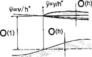
where /1* = hl(l, t) is an instantaneous relative distance of the edge vertex from its projection upon the ground. Parameter Z, as introduced previously, represents the arc coordinate measured along the planform contour. Note that due to assumption (2.1) both the wing and wake surfaces have spanwise and chordwise slopes of the order of О(h0). Therefore, the edge flow problem formulation can be linearized. In fact, as prescribed by (2.1), in the stretched local region De the distances of points on the wing’s upper and lower surfaces from the horizontal line у = 1, as well as the distances of points of the ground surface from horizontal line у = 0 are of the order of О(h0) (see Fig. 2.4). Therefrom with an asymptotic error of the order of О (ft^), the tangency conditions on the wing and on the ground can be transferred to horizontal lines у — 0 and у — 1, respectively.

The corresponding problem for the leading (side) edge flow velocity po­tential (pe = (fe can be formulated as follows:

Parameters gZu, gZi, and dg depend on arc coordinate Z and time t and have to be determined in the process of matching with the asymptotic solutions constructed in the upper and channel flow regions. Note that without loss

of generality, it is possible to set dg = 0. In the problem for the flow near a leading edge, the boundary conditions at infinity on the wake and at the trailing edge have been lost. Their influence on the leading edge flow will be recovered by matching with the asymptotic descriptions of the velocity potential in the channel and upper flow regions.

Due to the linearity of the local problem, its general solution can be presented in the form

<fle = Gl^o^ae + + 0*3 + &4^о? (2.39)

where di are parameters to be determined through matching. Function </?ae is a homogeneous solution, satisfying the condition of no normal velocity on the wing and ground surfaces (du = d = dg = 0). This homogeneous solution corresponds to a circulatory flow around the edge. Function (ръе represents a nonhomogeneous solution, which is generated by a prescribed normal velocity upon the wing and the ground. Both </?ae and <РЬе are of the order of 0(1). Linear combination a^hQv + <24 automatically satisfies the Laplace equation and does not violate the flow tangency condition on solid boundaries.

We turn to determination of functions <pae and <рье- To find solution of the homogeneous problem for the flow past the leading (side) edge, we perform a conformal mapping of the local flow domain De onto the upper half plane

= 77 > 0 of the auxiliary complex plane ( = £ + і r) by the Christoffel – Schwartz integral; see Lavrent’ev and Shabat [129]. The correspondence of points in the physical plane (i = v + і у and auxiliary plane ( is illustrated in Fig. 2.5.

The mapping function has the form

li = — (1 + C + lnC)> (2.40)

7Г

where і = д/—Ї is an imaginary unit. For purely circulatory flow around the edge in the plane of the complex potential /ae = <£ae + i^ae, the flow with unit velocity at the left infinity v = – 00 is represented by a strip of unit width. Conformal mapping of this strip onto the upper half plane > 0 is realized by the function

/ae = ^ae "b І Фа-е ~ in £. (2.41)

7Г

Eventually, the solution of the homogeneous problem is given by the formulas (2.40) and (2.41). Excluding the auxiliary variable £, we obtain the following relationship between the “physical” complex plane Д = z/+i у and the complex potential /ae = </?ae + і Фае, representing the homogeneous component of the problem solution.

тгД = 1 + ехр(тг/ае) + тг/ае. (2.42)

The flow pattern, corresponding to the homogeneous solution (pae is depicted schematically in Fig. 2.6. At points on the wing surface near the leading (side) edge, where Де = v? ae + і, /і = v + i, v < 0, the potential (pae can be determined through the following implicit relationship:

ТГй = 1- ЄХр(7Г(/?ае) + ТГ^ае-

It can be shown that the flow velocity has a standard square root singularity at the leading edge. In fact, in the immediate vicinity of the edge vertex v —> 0 — 0, (pae —> 0, and it follows from the expansion of equation (2.43) that

I 1

TTP~ 1 – (1 + TT^ae + ^Vae + ‘ ‘ ‘) + ^ae ^ (2‘44)

wherefrom for и —у 0 — 0,

ss0′ (245)

To match the flow potentials in regions Du and D, one needs the asymp­totic representations of the edge flow potential (pae far from the edge. Turning to the variable v = h*ei> = h0h*ev and setting h0 to zero for fixed v — 0(1), one obtains

• on the upper surface of the wing (v — v/h*e —> — oo, у — 1 + 0),

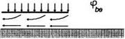Fig. 2.6. Flow patterns corresponding to the homogeneous (fae and nonhomogeneous <ръе components of the edge flow potential.

(2.47)

We turn to the determination of the nonhomogeneous solution </?be – Using the same mapping function (2.41), one comes to the following problem for a complex conjugate velocity Wbe = ^be — i^be in the auxiliary plane £: Find an analytic function u>be(C) in the upper half plane = r] > 0 in terms of its imaginary part Эгиье — —^be given on the axis £ (see Fig. 2.7).

It can be verified that the following expression satisfies the problem under consideration:

Wbe = – [(du – di)ln(l + C) + d In £]. (2.48)

7Г

At points on the wing in the vicinity of the edge (£ = £ < 0),

ube = SRu>be = l[(du — di) In |1 + ^| + diln|^|]. (2.49)

7Г

The velocity potential corresponding to the nonhomogeneous solution can be derived by means by integrating(2.49):

^be = Uhedv. (2.50)

Jo

At points on the wing surface, the auxiliary variable £ = Щ is related to the variable v in the following way:

тгі/ = 1 + £ + 1п|£|, £ < 0. (2.51)

The flow pattern corresponding to a nonhomogeneous solution is presented schematically in Fig. 2.6. In the particular case of an infinitely thin edge (zero vertex angle du = d — d 3), the following expression for (ръе can be derived from the previous more general relationships:

To match the edge flow potential with the velocity potentials in regions Du and D, we need to know asymptotic representations of ще and c^be far from the leading (side) edge. These can be found in the form

• on the lower surface of the wing (v —» —oo, у = 1 — 0, £ —0 — 0)

(2.55)

Taking into account expressions (2.39) and (2.45) we obtain the following estimate of the behavior of the velocity near the leading edge of the lifting surface along the normal to the planform contour:

where the “minus” sign corresponds to the upper surface of the wing, and the “plus” sign corresponds to the lower surface of the wing. Formula (2.57) is useful for calculating the suction force at the leading edge of the lifting system in both steady and unsteady motion.

Note that the asymptotic solution of the problem for the flow near the edge of a vortex sheet in the extreme ground effect has the same structure as that for an infinitely thin leading (side) edge.

Near the trailing edge /2, the velocity potential ipe = ipte should sat­isfy not only the flow tangency conditions on the wing and the ground but also comply with the dynamic and kinematic conditions on the vortex sheet emanating from the wing due to unsteady and three-dimensional effects. Ex­cluding the homogeneous component of expression (2.39) which incorporates a square root singularity for the flow velocity at the edge, we can write the velocity potential ipte for the flow in the vicinity of the trailing edge in the form

<Pte = Mo^be + b2hlv + b3h0,

where v = v/h*(l, t) = vjh^ and y>be is given by the formula

(Phe= Ще dP, (2.59)

Jo

Ще = ^[(eu – ei) In |1 + f | + e In |£|]. (2.60)

The auxiliary variable £ is related to v by equation (2.51). Parameters eu, e and bi, 62, bs are unknown and have to be determined by asymptotic match­ing. It is essential to note that parameters 62 and 63 have different magnitudes on the upper (y = y/h*e = 1 + 0) and lower (y = y/h*e = 1—0) surfaces of the vortex sheet behind the trailing edge, i. e., Ф b^ and 63 ф b% . This is caused by the jump discontinuity of the velocity potential and the tangential velocity at the trailing edge I2, the latter in the case of unsteady flow. At the same time, the solution satisfies the condition of the continuity of the normal velocity component across the vortex sheet. In the particular case of an infinitely thin trailing edge (zero vertex angle eu = e = e), it follows from (2.59) and (2.60) that

є 1

<РЪе = ~ ^(тг^ае – 1) – o^ae]- (2-61)

7Г Z

The asymptotic representation of иъе and сръе far from the trailing edge can be found from expressions (2.53)-(2.56) by replacing duд by еид and h*e by h*e. Note that the solutions of local flow problems, presented above, lose validity in the vicinity of the order of О(h0) of the corner points of con­tours 11,^2, where the flow is essentially three-dimensional. Near such corner points, additional solutions should be constructed, but this question will not be discussed here.

In the upper flow field Du, where (x, г/, г) = 0(1) for h0 —> 0 and є = O(/i0), both the wing and the wake approach the ground. In the limit, one comes in the upper half space to the problem for the flow, generated by the tangency conditions on the upper surfaces of the wing and the wake. Because є tends to zero (which practically means that, e. g., the relative ground clearance, angle of attack, curvature and thickness of the wing are small) the upper flow can be linearized, so that tangency conditions are satisfied upon the projections of the wing and wake sheet onto the plane у = 0.

In the region Du, we seek the upper flow perturbed velocity potential in the form

<Pu = h0<Pu1(x, y,z, t) + O(h%), <pUl= 0(1). (2.25)

Substitution of this expansion in the flow problem (2.2-2.6) leads to the following equation and boundary conditions for the upper flow problem:

where au = au//i0,aWl = aWl/h0. The channel flow and edge flow descrip­tions are lost in Du. Their influence will be recovered by asymptotic matching of the upper flow potential with that of the channel flow through edge regions.

Note that the boundary condition on the upper surface of the wake vortex sheet may be formulated as the flow tangency condition if the downwash olwx = ho&wx in the wake is known.

The upper flow potential (pUl is constructed in the form

The first term of (2.31) represents the induced velocity potential of the source-sink distribution along the contours of the leading and side edges of the wing li and the edges of the wake /3. This contour distribution charac­terizes the influence of the channel flow upon the upper flow due to leakage of air from under the wing. The strength of the contour sources (sinks) Q(l, t) is determined as a result of matching the upper and channel flow potential through edges l and /3. The second and third terms of (2.31) correspond to the potential of the surface distributions of sources and the sinks of strength —2au upon S and —2aWl upon W. The latter result is based on a thin body theory.

Near the edges l and I2, the function ipUl has the following asymptotic representations:

where l is the arc coordinate measured along the planform contour, v is the external normal to the planform, and ( auw) = au(l, t) — aw(Z,£) is the jump of downwash on the upper surface of the wing across the trailing edge I2, (aUw) = (otUw)/h0. Parameters Ai, A2 and J5i, J52 characterize the influence of distant sources.

In the region Д, where ~ ifi, x = 0(1), z = 0(1), and у = O(h0), we introduce stretching of the vertical coordinate

(2.7)

In the channel flow region, both the condition at infinity (decay of pertur­bations in three-dimensional flow) and the Kutta-Zhukovsky condition at the trailing edge are lost. The influence of these conditions will be transmitted to the channel flow region by matching with the asymptotic solutions to be obtained in regions De and Du.

We seek <p in the form of the following asymptotic expansion:

<P і = Vi+f^Vi* = <Ph+<Pi2 К ln^- + <Ph h0 + h%<p**, {(fix, <p**) = 0(1),

° (2.П)

which can be shown to satisfy the requirement of matching of the asymptotic representations of the velocity potential in the regions Д, £)u, and De. Sub­stituting (2.11) in (2.8), yields the following equations for the functions <p* and <p**:

= 0, (x, y, z) Є A; (2.12)

Then, using the same asymptotic expansion (2.11) in the flow tangency con­ditions on the lower surface of the wing (2.9) and on the ground (2.10), we obtain the following set of equations:

• on the lower surface of the wing

Integrating (2.12) two times with respect to у and accounting for (2.14) and (2.16), we obtain an important conclusion: with an asymptotic error of the order of O(h0), the description of the channel flow is two­dimensional in the plane parallel to an unperturbed position of the ground surface, i. e., to the plane у = 0,

<P* = ¥>*

Integrating (2.13) one time with respect to у, gives

where /**(x, z) is an unknown function. Taking into account equations (2.15) and (2.17), we obtain

Substracting (2.21) from (2.20), we obtain the following channel flow equa­tion:

where h* = h*(x, z,t)/h0 = y – yg, h*(x, z) = y(x, z) – yg{x, z) is the instantaneous distribution of the gap between the wing and the ground.

Thus, it has been shown that for very small clearances (an extreme ground effect), the flow field under the wing in the ground effect has a two-dimensional description and its perturbation velocity po­tential ~ (p* satisfies quasi-harmonic equation (2.22) in a two­dimensional domain S bounded by the wing planform contour.

The boundary conditions for (p* at the leading l and trailing edges I2 of the lifting surface will be obtained by matching.

From a physical viewpoint, equation (2.22) can be interpreted as the equa­tion of mass conservation in a highly constrained channel flow region with
known distributed mass addition due to tangency conditions on the lower surface of the wing and part of the ground situated under the wing.

For channel flow under the wake, the same procedures can be used to relate the induced downwash aw = O(h0) in the wake,

qw = = h0 + ^W2 In 7 + ^w3) (2.23)

to the wake channel flow potential <p[7] and the corresponding instantaneous gap distribution h^(x, z) = yw(x, z, t) – yg(x, z, t) by the following equation:

where = (yw – yg)/h0 = 2/w – 2/g.

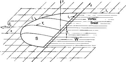
1.2 Formulation of the Three-Dimensional Unsteady Flow Problem

Consider a wing of small thickness and curvature, performing an unsteady motion above a solid nonplanar underlying surface in an ideal incompressible fluid[5] (see Fig. 2.1). Assume that motion of the wing is the result of super­position of the main translational motion with variable speed U(t) and small vertical motions due to heave, pitch, and possible deformations of the lifting surface. Introduce a moving coordinate system in which the axes x and z are located upon an unperturbed position of the underlying boundary (the ground). Axis x is directed forward in the plane of symmetry of the wing, and axis у is directed upward and passes through the trailing edge of the root chord.

In what follows, all quantities and functions will be rendered nondimen­sional by using the root chord C0 and a certain characteristic speed U0. De­fine the relative ground clearance h0 as the ratio of the characteristic dis­tance of the trailing edge of the wing’s root section from the unperturbed position of the ground to the length of the root chord. Introduce functions t/u(x, z, t), y(x, z, t), yg(x, z, t), and yw(x, z,t), characterizing, respectively, the instantaneous positions of the upper and lower surfaces of the wing, the surfaces of the ground, and the wake from the plane у — 0.

Introduce a small parameter є, characterizing a perturbation (for example, angle of pitch, curvature, thickness, amplitude of oscillations or deformations of the wing, deformation of the ground surface, etc.).

With the intention of developing an asymptotic theory valid in close prox­imity to the ground, suppose that the relative ground clearance is small, that is, h0 1. Assume that at any moment the instantaneous distances of points of the wing, wake, and ground surfaces from the plane у = 0 are of the same order as h0 and are changing smoothly in longitudinal and lateral directions. Thus, if y(x, z,t) describes either of these surfaces, then

(!”l’S)=o(£)=ow<<L <2л)

It should be noted that in the case of the extreme ground effect, the assump­tion adopted є = O(h0) does not mean that flow perturbations are necessarily small. It will be shown later on that in the extreme ground effect, the input of the order of О(є) can result in the system’s response of the order of 0(1).

The inviscid incompressible flow around a wing in the ground effect is governed by the three-dimensional Laplace equation and is subject to

• the flow tangency condition on the surfaces of the wing and the ground,

• the dynamic and kinematic conditions on the wake surface (pressure and normal velocity should be continuous across the wake), and

• the decay of perturbations at infinity.

The Kutta-Zhukovsky requirement of pressure continuity can be specified at the trailing edge, although it is automatically satisfied through the boundary conditions on the wake surface.

With this in mind, one can write the following flow problem formulation with respect to the perturbation potential

dx2 dy2 + dz2 ’

ftp = <ty _ u(fs] %.,! dip dyUti %,,!

dy Idx UJ dx dz dz dt ’

У = yu,(x, z,t), (x, z)eS; (2.3)

_ Гrr/#xl дУе, dipdyz, dyg. dx dx + dz dz + dt’

y = yg(x, z,t), (x, z) Є G; (2.4)

(Vipn) =(Vipn) + , y = yw(x, z,t), (x, z) £ W; (2.5)

—> 0, x2 + y2 + z2 -> oo, (2.6)

where 5, G, and W are the areas of the wing, the ground, and the wake related to the square of the root chord.

According to the technique of matched asymptotics, the flow domain will be subdivided into the following subdomains with different characteristic length scales (see Fig. 2.2, where, for simplicity, the subdivision is illustrated in two dimensions):

• the upper flow region Du above the wing, its wake and part of the ground outside the projection of the wing and the wake upon the unperturbed ground plane;

• the channel (lower) flow region D under the wing and the wake;

• the edge flow regions De in the vicinity of the edges of the lifting surface and the wake.

In each of the regions, asymptotic solutions of the problem (2.2)-(2.6) are constructed for h0 —» 0 in appropriately scaled coordinates.

The asymptotic matching and additive composition of these solutions en­able accounting for the interaction of different parts of the flow and obtaining a uniformly valid solution for the entire flow domain. In what follows, con­sideration is restricted to the asymptotic accuracy of the order of O(h0).

With the increasing power of computers, it becomes possible to study the aerodynamics of wing-in-ground-effect vehicles by direct numerical modelling on the basis of appropriate viscous flow problem formulations. Similar to computational methods based on Euler equations, this approach enables suf­ficiently rigorous representation of the geometry of the vehicle. Besides, such a technique is not constrained by technical difficuties related to simultaneous physical modelling by using several similarity criteria (say, Froude number and Reynolds number). It is not restricted either in ranges of variation of the said criteria, so that the future of full scale numerical modelling looks promising.

However, practically, the implementation of numerical approaches intro­duces certain difficulties. First of all, the numerical treatment of viscous flows for large magnitudes of the Reynolds number is associated with the necessity of solving the Navier-Stokes equations with a very small parameter in front of the higher derivative. This fact gives birth to numerical instabilities due to ill conditioning of corresponding matrices and considerably complicates computations even in two dimensions. The difficulties multiply for the case of unsteady, three-dimensional flow.

An approximate method for computing ground-effect lifting flows with rear separation was proposed by Jacob [116]. The author used an iterative approach combining the three-dimensional lifting surface theory for inviscid incompressible flow with a two-dimensional flow model incorporating com­pressibility and displacement effects. The author’s analysis implicitly contains an assumption that the aspect ratio of the wing is moderate or large.

Kawamura and Kubo [117] used a finite-difference method to solve a 3-D incompressible viscous flow problem for a thin rectangular wing with end- plates moving near the ground plane. They employed the standard MAC method (implying the use of the Poisson equation for the pressure and the Navier-Stokes equations) and a third-order upwind scheme. They did not use any turbulence closure models and restricted their calculations to Re — 2000.

Akimoto et al. [118] applied a finite-volume method to study the aerody­namic characteristics of three foils in a steady two-dimensional viscous flow on the basis of the Navier-Stokes equations with the Baldwin-Lomax turbu­lence model. To provide modelling of the wake, the position of its centerline was determined by a numerical streamer. The centerline of the wake was rep­resented by a line of segments, extending from the trailing edge of the foil to the boundary of the computational domain. The number of finite volumes used in the calculation was 30×120 in vertical and longitudinal directions, re­spectively. All calculations were carried out for a Reynolds number equal to 3 x 106. The authors report that the typical CPU time for a set of parameters was of the order of 150 minutes on an alpha-chip workstation.

Steinbach and Jacob [119] presented some computational data for the air­foils in a steady ground effect at a high Reynolds number. Their approach was based upon an iterative procedure including the potential panel, boundary layer integral method and the rear separation displacement model.

In 1993 Hsiun and Chen solved the steady 2-D incompressible Navier- Stokes equations for laminar flow past an airfoil in the ground effect. Later on [120], the same authors developed a numerical scheme based on a stan­dard к — є turbulence model, generalized body fixed coordinates, and the finite volume method. They presented some numerical results concerning the influence of Reynolds number, ground clearance, and angle of attack on the aerodynamics of a NACA 4412 airfoil. The range of Reynolds numbers there­with did not exceed 2 x 106.

The Reynolds averaged Navier-Stokes (RANS) approach was also applied by Kim and Shin [121] to treat a steady two-dimensional flow past different foils, including NACA 6409, NACA 0009, and an S-shaped foil, the latter form providing static stability of longitudinal motion. Transformed momen­tum transport equations were integrated in time using the Euler implicit method. A third-order upwind-biased scheme was used for convection terms, and diffusion terms were represented by using of a second-order central differ­ence scheme. The pressure field was obtained by solving the pressure Poisson equation. Since a nonstaggered grid was adopted in this method, the fourth – order dissipation term was added in the Poisson equation to avoid oscillation in the pressure field. Two-block H-grid topology was adopted both above and below the foil surface. Two grid points from each block overlapped to ensure flow continuity. For a Reynolds number of 2.37 x 105 adopted for calculations and a 150×120 grid, employed to simulate turbulent flow, 300-500 seconds were required to produce a calculation on Cray C-90 supercomputer.

Hirata and Kodama [122] performed a viscous flow computation for a rectangular wing with endplates in the ground effect. For this purpose, they used a Navier-Stokes solver, based on a third-order accurate upwing differ­encing, finite-volume, pseudocompressibility scheme with an algebraic turbu­lence model to close the system of equations. To be able to treat complex configuration of the flow the, authors used a multiblock grid approach.

Hirata [123] extended the same technique to attack numerically the prob­lem for a power-augmented ram wing (PARWIG)-in-ground effect. The thrust of the propeller, ensuring power augmentation, was represented by prescribed body-force distributions. However, the Reynolds number for which the cal­culations were made was somewhat moderate (Re = 2.4 x 105). A similar approach was used by Hirata and Hino [124] to treat the aerodynamics of a ram wing of finite aspect ratio.

Barber et al. [125] applied RANS equations with а к — є turbulence model to investigate the influence of a boundary condition on the ground on the resulting calculated aerodynamic characteristics of a foil in two-dimensional viscous flow. The authors aimed at discerning differences in the existing mod­elling technique of ground effect aerodynamics. Calculated results were pre­sented for Re = 8.2 x 106. In another paper by the same authors [126], the RANS technique was used to analyze the deformation of an air-water inter­face, caused by a wing flying above the water surface.

It should be noted that the application of computational fluid dynamics (CFD) at very high Reynolds numbers is not straightforward for both numer­ical and physical reasons; see Patel [127] and Larsson et al. [128]. The general problem is that the ratio of the smallest to the largest scales of the flow decreases with an increase in the Reynolds number. Numerically, it means that more grid points are required to obtain a given resolution and physically the nature of turbulence changes, which means that turbulence models de­veloped at low Reynolds numbers might not be valid for high ones. Viscous effects are comparable with inertial ones in the immediate vicinity of the wall. Therefrom, for sufficient resolution, the number of points of the grid in the direction normal to the surface of the body should be much larger than along that surface. As a result, as a consequence of limited computer resources, extremely elongated numerical cells appear near the body surface, causing ill conditioning of corresponding systems of equations and breakdown of most of the solvers; see Larsson [128]. In spite of the progress envisaged in numeri­cal solution of Navier-Stokes equations with the use of large eddy simulation (LES), and ultimately through direct numerical simulation (DNS), the ex­perts do not expect that these methods would be realized earlier than 10 and 20 years, respectively.

Efremov [104] used a collocation method to solve numerically the integral equation describing oscillations of a flat plate of infinite aspect ratio in motion near the interface of fluids of different densities.

Gur-Milner [105] used a continuous representation of loading with a Birnbaum-Prantdtl double series to calculate the steady and unsteady char­acteristics of wings of arbitrary planform near the ground within the frame­work of linear theory.

Vasil’eva et al. [106] formulated a three-dimensional linearized unsteady theory of a lifting surface moving in the presence of a boundary of two media with different densities. The authors were able to calculate the aerodynamic derivatives for unsteady motions of the lifting surface of a given planform. In particular, they performed calculations for an air-water interface, concluding that, within the assumptions of the mathematical model adopted, the surface of water under a wing behaves as if it were a solid wall.

Avvakumov [107] performed calculations of the aerodynamic derivatives of a wing of finite aspect ratio in motion above the a wavy wall surface, using the vortex lattice method to model the unsteady aerodynamics of the lifting system and the distribution of three-dimensional sources on the underlying surface.

A 2-D estimate of what the authors designate “dynamic ground effect” was made by Chen and Schweikhard [108] by using of the method of discrete vortices of such transitional maneuvers of a flat plate airfoil as descent or climb. In this work, a simplifying assumption was made that the foil unsteady vortex wake is directed along the flight path.

A 3-D numerical simulation of the aerodynamics of wings of finite thick­ness in the ground effect was carried out by Nuhait and Mook [109, 110], Mook and Nuhait [111], Elzebda et al.[112], and Nuhait and Zedan [113]. In these works, the authors employed the vortex lattice method and modelled the shedding of the vorticity into the wake by imposing the Kutta-Zhukovsky condition along the trailing edges and wing tips. The position and distribu­tion of the vorticity in the wake were determined by requiring the wake to be force free. The model is not restricted by planform, camber, angle of pitch, roll, or yaw as long as stall and vortex bursting do not occur. The method is sufficiently general, and the authors gave calculated examples of the unsteady ground effect related to the descent of the wing and performed computations of the steady-state aerodynamics of wings and wing-tail combinations.

Ando and Ishikawa [114] investigated the aerodynamic response of a thin airfoil at zero pitch angle moving in proximity to a wavy wall which advances in the same direction but with different speed. The authors showed that the wavelength and speed of advancement have considerable influence on what they called “the second-order ground effect.”

Kornev and Treshkov [115] developed an approximate method for calcu­lating the aerodynamic derivatives of a complex lifting configuration based on the vortex lattice approach and the linearization of the unsteady flow com­ponents in the vicinity of a nonlinear steady state of the system. They made some numerical estimates of the contribution of different nonlinear factors to the aerodynamics of wing-in-ground-effect craft.

Belotserkovsky’s monograph “Thin Wings in Subsonic Flow” published in 1965 [80], became a standard for vortex lattice methods applications. It con­tains a set of results on rectangular wings flying over a solid boundary ob­tained within linear theory. Later on, vortex lattice methods were successfully applied to numerical solutions of nonlinear problems of aerodynamics of lift­ing systems; see Belotserkovsky et al. [81, 82].

The linearized vortex lattice approach was used by Farberov and Plissov [83], Plissov [84], and Konov [85, 86] to determine the characteristics of wings of different planforms and lateral cross section near the interface, and by Plissov and Latypov [87] to compose tables of rotational derivatives for wings of different aspect ratios near the ground. Ermolenko [88] conceived an ap­proximate nonlinear approach to the steady aerodynamics of wings near a solid boundary based on iteration of position of trailing vortices in connec­tion with the induced velocity field in a plane, normal to the wing and passing through the trailing edge.

Treschevskiy and Yushin [89], Pavlovets et al. [90], Yushin [91], and Volkov et al. [92] utilized various modifications of discrete and panel vortex methods to compute the characteristics of wings and wing systems in the ground effect.

Katz [93] used a vortex lattice method incorporating a freely deforming wake to investigate the performance of lifting surfaces close to the ground with application to the aerodynamics of racing cars.

Deese and Agarval [94] employed an Euler solver, based on the finite – volume Runge-Kutta time-stepping scheme to predict the 3-D compressible flow around airfoils and wings in the ground effect. They applied this tech­nique to calculate the aerodynamics of Clark-Y airfoil (infinite aspect ratio) and a low-aspect-ratio wing with a Clark-Y cross section.

Kataoka et al. [95] extended the two-dimensional steady-state approach to treat the aerodynamics of a foil moving in the presence of a water surface. The foil was replaced by a source distribution on its contour and a vortex distribution on its camber line. The free surface effect was taken into account by distributing wave sources on an unperturbed position of the boundary. Mizutani and Suzuki [96] used an iterative approach based on panel meth­ods for the airflow field and the Rankine method for the water flow field to account for the free surface effects and calculated wave patterns generated by a rectangular wing with endplates. In both of these works, the differences in the aerodynamic predictions for a wing near a free surface and near a corresponding solid boundary were found to be insignificant.

By using the method of continuous vortex layers (vortex panel approach ), Volkov [97] carried out some computational investigation into the influence of the geometry of the foil upon its aerodynamic characteristics in proximity to the ground.

Morishita and Tezuka [98] presented some numerical data on the two­dimensional aerodynamics of the airfoil in the compressible ground-effect flow.

Day and Doctors [99] applied the vortex lattice method to calculate the steady aerodynamic characteristics of wings and wing systems in the ground effect with the incorporation of the deformation of the wakes into the numer­ical scheme.

Chun et al. [100] carried out computations for the aerodynamic charac­teristics of both isolated wings and the entire craft of the flying wing configu­ration in ground effect using the potential-based panel method of dipole and source distributions. Standingford and Tuck [101] applied the high-resolution approach developed within the steady lifting surface theory to investigate the influence of endplates upon the characteristics of a thin flat rectangular wing in the ground effect. The authors report this approach yields better accuracy than the standard vortex lattice method near the edges of a junction of a wing-plus-endplates system.

Hsiun and Chen [102] proposed a numerical procedure for the design of two-dimensional airofoils in the ground effect. The corresponding inverse problem was based upon the least square fitting of a prescribed pressure distribution and a vortex panel method to obtain a direct solution of the problem.

Design problems for airfoil sections near the ground have also been con­sidered by Kiihmstedt and Milbradt [103], whose objectives for optimization were stability and maximum lift. These authors used and compared several potential code methods in both 2-D and 3-D formulations.