Category AERODYNAMICS OF THE AIRPLANE

The lift distribution over the span is defined in analogy to Eq. (2-9b) as

dL = сг{у)с{у)ч dy (3-12)

Here the local lift coefficient has been introduced in analogy to Eq. (2-10) as Ф) & —Су} (y)[12] The lift distribution of a wing in symmetric incident flow is shown in Fig. 3-5b. Finally, in Fig. 3-6 there is also shown the distribution of measured local lift coefficients сг over the span of a rectangular wing at various angles of attack.

By integrating Eq. (3-12) over the span, the total lift L and further, with Eq. (1-21), the lift coefficient are determined as

Cl==a^ = a f c&Wy)dy (3-13)

-s

Only single wings will be treated in this book. Wing systems such as, for example, biplane and tandem arrangements or ring wings (tube-shaped cylindrical surfaces) will not be considered.

In progress reports, more recent results and the understanding of the aerodynamics of the wing are presented for certain time periods, among others, by Schlichting [72, 74], Sears [78], Weissinger [97], Gersten [20], Blenk [7], Ashley et al. [2], Kiichemann [49], and Hummel [35]. The very comprehensive compilation of experimental data on the aerodynamics of lift of wings of Hoerner and Borst [31] must also be mentioned.

Figure 3-4 Most important geometric wing data of actual airplanes vs. Mach number. Evolution from subsonic to supersonic air­planes. {a) Profile thickness ratio 5 — tjc. (b) Aspect ratio A. (c) Sweepback angle of wing leading edge MaCI = drag-critical Mach number (see Sec. 4-3-4).

Figure 3-5 Illustration of lift distribution of wings, (a) Geometric designations, (b) Lift distribution over span.

To convey a concept of the various wing shapes that have actually been used in airplanes, the. profile thickness ratio 5=t/c, the aspect ratio A = b2/A, and the sweepback angle of the leading edge ipf of some airplanes are plotted in Fig. 3-4 against the flight Mach number. The plots show a clear trend of profile thickness and aspect ratio in the transition from subsonic to supersonic airplanes.

The profile thickness ratio decreases sharply with increasing Mach number, reaching values of tjc = 0.04 for supersonic airplanes. The aspect ratios are particularly large in the subsonic range for long-distance airplanes but considerably smaller for maneuverable fighter planes. In the supersonic range, the implementation of larger aspect ratios is no longer required for aerodynamic reasons. In this range, therefore, design considerations have led to aspect ratios as small as A — 2. The sweepback angle is close to zero at low Mach numbers but increases to ^45° at high subsonic speeds. In the supersonic range, airplanes with both relatively large sweepback (tp/^60o) and small sweepback (^«30°) are found. Truckenbrodt [86] has shown to what extent the geometric wing data of Fig. 3-4 have been determined by a decisive understanding of the drag of wings.

3- 1 INTRODUCTION

For an airfoil of infinite span, the flow field is equal in all sections normal to the airfoil lateral axis. This two-dimensional flow has been treated in detail by profile theory in Chap. 2. For an airfoil of finite span as in Fig. 3-1, however, the flow is three-dimensional. As in Chap. 2, incompressible flow is presupposed.

2- 1-1 Wing Geometry

The wing of an aircraft can be described as a flat body of which one dimension (thickness) is very small in relation to the other dimensions (span and chord). In general, the wing has a plane of symmetry that coincides with the plane of symmetry of the aircraft. The, geometric form of the wing is essentially determined by the wing planform (taper and sweepback), the wing profile (thickness and camber), the twist, and the inclination or dihedral of the left and right halves of the wing with respect to each other (V form) (see Fig. 3-1). In what follows, the geometric parameters that are significant in connection with the aerodynamic characteristics of a lifting wing will be discussed.

For the description of wing geometry, a coordinate system in accordance with Fig. 3-1 that is fixed in the wing will be established with axes as follows:

x axis, wing longitudinal axis, positive to the rear

у axis, wing lateral axis, positive to the right when viewed in flight direction, and perpendicular to the plane of symmetry of the wing z axis, wing vertical axis, positive in the upward direction, perpendicular to the xy plane

У

Figure 3-1 Illustration of wing geometry. (a) Planform, xy plane, (b) Dihedral (V form), yz plane, (c) Profile, twist, xz plane.

It is expedient to select the position of the origin of the coordinates as suitable for each case. Frequently it is advisable to place the origin at the intersection of the leading edge with the inner or root section of the wing (Fig. 3-1), or at the geometric neutral point [Eq. (3-7)]. The wing planform is given in the xy plane; the twist, as well as the profile, in the xz plane; and the dihedral in the yz plane.

The largest dimension in the direction of the lateral axis (y axis) is called the span, which will be designated by b = 7s, where s represents the half-span. Frequently the coordinates will be made dimensionless by reference to the half-span s, and abbreviated notations

f = T	(3-U)
	(3-lb)
f = T	(3-lc)

are here introduced.

The dimension in the direction of the longitudinal axis (x axis) will be designated as the wing chord c(y), dependent on the lateral coordinate y. The wing chord of the root or inner section of the wing (y = 0) will be designated by cr, and the corresponding dimension for the tip or outer section by ct. In Fig. 3-2, the geometric dimensions are illustrated for a trapezoidal, a triangular, and an elliptic planform.

For a wing of trapezoidal planform (Fig. 3-2a), an important geometric parameter is the wing taper, which is given by the ratio of the tip chord to the root chord:
(3-2)

A special case of the trapezoidal wing is the triangular wing with a straight trailing edge, also designated as a delta wing (Fig. 3-2b).

The wing area A (reference area) is understood to be the projection of the wing on the xy plane. For a variable wing chord, the area is obtained by integration of the wing chord distribution ciy) over the span b = 2s; that is,

(3-3)

Figure 3-2 Geometric designations of wings of various planforms. (a) Swept-back wing. (b) Delta wing, (c) Elliptic wing.

From the wing span b and the wing area A, there is obtained, as a measure for the wing fineness (slenderness) in span direction, the aspect ratio

II X|<s	(34a)
II if I»	(34b)
As mean chord and reference wing chord, especially for the introduction of dimensionless aerodynamic coefficients, the quantities
A cm=J	(3-5a)
s CjU = i fc2(y)dy	(3-5 b)
4

are used, where the ratio > 1. For the trapezoidal planform, it may be easily

demonstrated that the reference chord cM is equal to the local chord at the position of the center of gravity of the half-wing; that is, = c(yc) (Fig. 3-2a and b). The sweepback of a wing is understood to be the displacement of individual wing cross sections in the longitudinal direction (x direction). Representing the position of a wing planform reference line by x(y), the local sweepback angle of this line is

tan cp{y) = ^^~ (3-6)

If x(y) represents the connecting line of points of equal percentage rearward position, measured from the leading edge at the у section under consideration, then this fact is designated by giving the percentage number as an index of the value x. Accordingly, the position of the quarter-chord line is designated by x2s(y)- For the sake of simplicity, the index will be omitted in the case of the sweepback angle of the quarter-chord-point line. For aerodynamic considerations, furthermore, the geometric neutral point plays a special role. Its coordinates are given by

S

= j f c(y) Z2 5 {y)dy 5 = 0 (3 -7)

– S

For a symmetric wing planform, the geometric neutral point may be demonstrated to be the center of gravity of the entire wing area, whose quarter-chord-point line is overlaid by a weight distribution that is proportional to the local wing chord. The rearward distance of the geometric neutral point of a wing with a swept straight quarter-chord-point line is equal to the rearward distance of the quarter-chord point of the wing section at the planform center of gravity of the half-wing. Since, for a trapezoidal wing, the wing chord at the center of gravity of the half-wing is equal to the reference chord cM, the geometric neutral point for this wing lies at the cM/4 point (see Fig. 3-2a and b).

Of particular importance is the delta wing, a triangular wing with a straight

trailing edge (Fig. 3-2b). For the geometric magnitudes of this wing, especially simple formulas are obtained:

b _ 2 b _ 3 = 4 x _ Cy

cm cr tan cm 3 ■XiV25 2

For a wing of elliptic planform as in Fig. 3-2c, the geometric quantities become

A further geometric magnitude related to the wing planform is the flap (control-surface) chord сДу). The flap-chord ratio is defined as the ratio of flap chord (control-surface chord) to wing chord:

c(y)

For the description of the whole wing, data on the relative positions of the profile sections are required at various stations in span direction. They are required in addition to the knowledge of wing planforms and wing profiles. The relative displacement in longitudinal direction is specified by the sweepback, the displace­ment in the direction of the vertical axis by the dihedral, and the rotation of the profiles against each other by the twist.

In what follows, the geometric twist e(y) is defined as the angle of the profile chord with the wing-fixed xy plane (Fig. 3-3).[11] For aerodynamic reasons, in most cases the twist angle is larger on the outside than on the inside. The dihedral determines the inclination of the left and the right wing-halves with respect to the

Figure 3-3 Illustration of geometric twist.

xy plane. Let z^sx, у) be the coordinates of the wing skeleton surface. Then the local V form at station x, у is given by

tan у {x, у) = – (3-11)

The partial differentiation is done by holding x constant. If the wing is twisted, it must be specified in addition at which station xp(y) the angle v is to be measured. According to Multhopp [61], the aerodynamically effective dihedral has to be taken approximately at the three-quarter point xp =x75.

A change of the flow in the very thin wall boundary layer may, under certain conditions, alter considerably the entire flow pattern around the body. A number of methods have been developed for boundary-layer control that, in some instances, have obtained importance for the aerodynamics of the airplane. The basic principles of boundary-layer control will be explained briefly in this section. In most cases, boundary-layer control is considered in the following contexts: elimination of separation for drag reduction or lift increase, or only change of the flow from laminar to turbulent, or maintaining of laminar flow. The various methods that have been investigated mainly experimentally, but also theoretically in some instances, can be highlighted as follows: boundary-layer acceleration (blowing into the boundary layer), boundary-layer suction, maintaining of laminar flow through proper profile shaping (laminar profile). A comprehensive survey of this field is given by Lachmann [36].

Boundary-layer acceleration A first possibility of avoiding separation is given by introducing new energy into the slowed-down fluid of the friction layer. This can be done either by discharging fluid from the body interior (Fig. 2-52a) or, in a simpler way, by taking the energy directly from the main flow. This method consists of injecting fluid of high pressure into the decelerated boundary layer through a slot (slotted wing, Fig. 2-52b). In either case, the velocity in the wall layer increases through energy addition and thus the danger of separation is removed. For practical applications of the method of fluid ejection as in Fig. 2-52a, particular care is required in designing the slot. Otherwise, the jet may disintegrate into vortices shortly after its discharge. More recently, extensive tests [46] have led to the method of discharging a jet at the trailing edge of the wing, which has proved to be

Figure 2-52 Various arrangements for boundary-layer control, (a) Blowing. (b) Slotted wing, (c) Suction.

very successful in raising the maximum lift (jet flap). The same benefit has been gained from blowing into the slot of a slotted wing.

A slotted wing (see Fig. 2-52Ъ) functions in the following way: On the front wing (slat) A-В, a boundary layer forms. The flow through the slot carries this layer out in the free stream before it separates. At large angles of attack, the steepest pressure rise and hence the greatest danger of separation occurs on the suction side of the slat. Starting at C, a new boundary layer is formed that may reach the trailing edge without separation. Hence, by means of wing slats, separation can be prevented up to much larger angles of attack, so that much larger lift coefficients can be obtained. In Fig. 2-53, polar diagrams (lift coefficient cL vs. drag coefficient Ci)) are given of a wing without and with a wing slat and with a rear flap. In the slot between main wing and rear flap (Fig. 2-52b), the processes are the same, in principle, as those in the front slot. The lift gain from a front slat and a rear flap is considerable. Further information on this item will be given in Chap. 8.

Boundary-layer suction Boundary-layer suction is applied for two purposes: to avoid separation and to maintain laminar flow (see Schlichting [53] and Eppler [15]). In the first case, the slowed-down portions of the boundary layer in a region of rising pressure are removed by suction through a slot (Fig. 2-52c) before they can cause flow separation. Behind the suction slot, a new boundary layer is formed that, again, can overcome a certain pressure rise. Separation may never take place if the slots are suitably arranged. This principle of boundary-layer removal by suction

v Figure 2-54 Drag (friction) coefficients of flat plate in parallel flow with homogeneous suction; cq = (—u0 )/£/«, = suction coefficient; —u0 = constant suction velocity. Curves 1, 2, and 3 without suction. 1, Laminar; 2, transition laminar-turbulent; 3, fully turbulent; 4, most effective suction.

was checked out for a circular cylinder by Prandtl as early as 1904 and has been investigated by Schrenk [58] for wing profiles.

In the second case, suction is applied for the reduction of friction drag of wings (see Goldstein [20]). This is. accomplished if suction causes a downstream shift of the laminar-turbulent transition point. For this purpose, it turned out to be more favorable to apply areawise-distributed (continuous) suction, for example, through porous walls rather than through slots. In this way the disturbances by the slots were avoided, which could have led to premature transition. That the flow can be kept laminar through suction may be seen from the fact that the friction layer becomes thinner when suction is applied and, therefore, has less of a tendency to turn turbulent. Also, the velocity profile of a laminar boundary layer with suction has a shape, compared with that of a layer without suction, that makes transition to turbulence less likely even when the boundary-layer thickness is equal in both cases.

Of particular interest is the drag law of the plate with homogeneous suction, as given in Fig. 2-54, because it is characteristic for the drag savings gained through suction-maintained laminar flow. In comparison, the drag law of the plate with a turbulent boundary layer (without suction) is added as curve (3). The drag savings that may actually be achieved cannot yet be derived. First, the limiting suction coefficient must be known, which is necessary to keep the boundary layer laminar—even for large Reynolds numbers. This minimum suction coefficient was determined as

CQcr = 1-2 • 10-4

up to the highest Reynolds numbers. This remarkably small value is included in Fig. 2-54 as “most favorable suction” (curve 4). The difference between curves 3 “turbulent” and 4 “most favorable” suction represents the optimum drag savings, In the Reynolds number range Re = 106 to 10s, they amount to about 70-80% of the fully turbulent drag.

It should be understood, however, that this saving does not take into account the power needed for the suction. Even when taking this power into account, however, the drag savings are still considerable.

Ackeret et al. [2] were the first investigators to prove experimentally that it is possible to hold the boundary layer laminar by suction. Some of their test results on a wing profile are given in Fig. 2-55. This wing profile was provided with a large number of slots. The considerable savings in drag, even including the blower power needed for the suction, is obvious. The favorable theoretical results about drag savings by maintaining laminar flow have been confirmed completely through investigations of Jones and Head [20] on wings with porous surface.

Boundary layer with blowing Another very efficient means of influencing the boundary layer is the tangential ejection of a thin jet at a separation point. This method has been applied very successfully to wings with trailing-edge flaps. By ejecting a thin jet at high speed at the nose of the deflected flap, flow separation from the flap can be avoided and hence lift can be increased considerably. The underlying physical principles are demonstrated in Fig. 2-56. At large deflections, the effectiveness of the flap as a lift-producing element is markedly reduced by flow separation (Fig. 2-56a). The lift of a wing with deflected flap does not reach at all the value that is predicted by the theory of inviscid flow. Flow separation from the flap and a resulting loss in lift may be avoided, however, by supplying the boundary layer with sufficient momentum. This is accomplished by a thin jet of high speed, tangential to the flap, introduced near the flap nose into the boundary layer (Fig.

2- 56b). The lift gain that can be realized through blowing is shown in Fig. 2-56c as

Figure 2-55 Reduction of drag coefficient of wing profiles by suction through slots, after Pfenninger [2]. (a) Optimum drag coefficient of wing with suction vs. Reynolds number, (b) Profile-drag polar.

Figure 2-56 Flap wing with blowing at the flap nose for increased maximum lift. (a) Flap airfoil without blowing, separated flow. (b) Flap airfoil with blowing, attached flow, (c) Pressure distribution.

the difference between the two pressure distributions. The effect of blow jets and jet flaps is discussed in more detail in Sec. 8-2-3. A synopsis of the increase of maximum lift of wings through boundary-layer control has been written by Schlichting [54].

Maintaining laminar flow through shaping Closely related to maintaining laminar flow through suction is maintaining a laminar boundary layer through proper shaping of the body. The goal is the same, namely, to reduce the friction drag by shifting the transition point downstream. Doetsch [12] was the first to demonstrate experimentally that considerable drag reductions can be obtained in the case of a wing profile whose maximum thickness is sufficiently far downstream (laminar profile). By shifting the maximum thickness downstream, the pressure minimum, and thus the laminar-turbulent transition point of the boundary layer, is also shifted downstream because, in general, the boundary layer remains laminar in the range of decreasing pressure. Only after the pressure rises does the flow turn turbulent. These conditions are shown in Fig. 2-57 by comparing a “normal wing” of a maximum thickness position of 0.3c and a laminar profile with a maximum thickness position of 0.45c. In the former case the pressure minimum lies at 0.1c, in the latter case at 0.65c. The drag diagram indicates that, in the Reynolds number range from 3 • 106

to 107, the drag of the laminar profile is only about one-half that of the normal profile. The aerodynamic properties of such laminar profiles have been investigated in much detail in the United States [1]. Practical application of laminar profiles is impeded particularly by the extraordinarily high demand on surface smoothness necessary to ensure that the conditions for maintaining laminar flow are not lost with surface roughness. The studies of Wortmann [75] and Eppler [14, 15] on the development of laminar profiles for glider planes should be men­tioned.

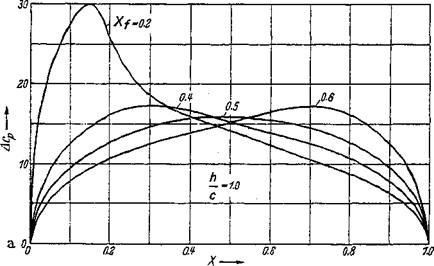
When the lift coefficient is small, the profile drag is caused essentially by friction. Its value depends on the position of the transition point and hence the lengths of laminar and turbulent stretches. The local velocities increase with angle of attack, leading to a slight rise of the profile-drag coefficient cDp. A further contributing factor is the increasing length of the turbulent boundary layer with a simultaneous shrinking of the length of the laminar layer. In the cLmax range, the profile drag rises steeply because of the strong increase in pressure drag caused by local separation. The Reynolds number has a very strong influence on the magnitude of the profile drag because both the pressure drag and the friction drag decrease with increasing Reynolds number (see Fig. 2-39b).

The dependence of the minimum drag coefficient cDmin on the Reynolds number [29] is plotted in Fig. 249 for several four-digit NACA profiles. Laminar separation causes quite high values of the minimum profile drag cDmin for small Reynolds numbers (Re <5 • 105). Symmetric profiles produce minimum drag at cL — 0, cambered profiles at the angle of smooth leading-edge flow. The value of cDmin decreases strongly when the Reynolds number grows. As soon as fully attached flow is established, the trend of the cDm-m curve is similar to that of the friction drag of the flat plate (see Fig. 248). In this range of Reynolds numbers (Re >8 • 10s), the minimum drag coefficient is raised more and more above the value of friction drag when the profile thickness grows (Fig. 249<z). The same behavior is found for the camber (Fig. 249b).

Peculiarities of the drag appear at laminar profiles (see Wortmann [75]). As an example, three-component measurements on the NACA 662 415 profile are plotted in Fig. 2-50 for various Reynolds numbers (after [29]). Over a limited range of small lift coefficients, the profile drag is constant, independent of the angle of attack. It is lower than that of a normal profile if the Reynolds number is large enough to prevent laminar separation. When the Reynolds number grows, cDp decreases; at the same time the dip in the drag curve, that is, the lift range for

mo

Figure 2-48 The friction law of the smooth flat plate (one wetted surface only) at zero incidence. Comparison of theory and experiment. Drag coefficient: Cf^D/q^bc. Theoretical curves: 1, laminar (Blasius); 2. turbulent (Prandtl); 3, turbulent (Prandtl, Sehlichting); 2a, transition laminar-turbulent (Prandtl); 4, turbulent (Schultz-Grunow).

Figure 249 Minimum drag of four-digit NACA profiles vs, Reynolds number, (a) Effect of thickness ratio. 0) Effect of camber ratio.

minimum drag, becomes narrower. When the angle of attack is increased, the pressure minimum shifts toward the nose and, in general, the transition point jumps upstream abruptly, causing a very strong increase in profile drag. This process is observed at reduced a when Re increases and at last, at very large Reynolds numbers, the dip in the drag curve disappears completely. A normal polar curve with an elevated Сдтin takes over (see [50]).

Computational determination of profile drag The profile drag of lifting wings can be determined theoretically by means of boundary-layer theory as long as the flow

Figure 2-50 Three-component measurements on the laminar profile NACA 662-415 at various Reynolds numbers.

is fully attached. Pretsch [48] and Squire and Young [62] were the first investigators to publish such methods, which were later improved by Cebeci and Smith [9]. The profile drag (= pressure drag plus friction drag) is obtained from the velocity distribution in the wake at large distance from the body in the form

+ CO

DP = oh f u(Uсо – u) dу (2-117)

// = – со

Here, b is the span of the wing profile, у is the coordinate normal to the incident flow direction, and u(y) is the velocity distribution in the wake. By defining the profile drag coefficient cDp by Dp = cDpbc(o/2)Ul, and introducing the momentum thickness 52oo, the drag of both sides of the profile with a fully turbulent boundary layer is given as

g

cDp = 2-у1 (2-1 l&z)

Here Re = uxcfv is the Reynolds number and U(x) is the velocity distribution over the profile as obtained for potential flow. The second relationship [Eq. (2-118b)] is derived from the findings of boundary-layer theory (see Schlichting [55]). For a plate in parallel flow, there is U(x) = UX= const.

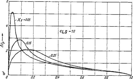
For some symmetric wing profiles in chord-parallel flow, the coefficients for the profile drag from [62] are summarized in Fig. 2-51. The profile thickness varies from t/c = 0 (flat plate) to t/c = 0.25 and the Reynolds number ranges from Re = 106 to 108. The profile drag is strongly dependent on the location of the laminar-turbulent transition point xtT, which varies from xtr/c = 0 to 0.4. The increase in profile drag with thickness must be attributed essentially to a rising pressure drag.

Truckenbrodt [48] extended the drag formula, Eq. (2-118b), to contain explicitly the profile shape instead of the velocity distribution of potential flow. Application of this method to a large number of NACA profiles produces the simple relationship between the profile-drag coefficient and the thickness ratio tjc,

cDp 2Cft

Here Cft is the drag coefficient of the flat plate with a fully turbulent boundary layer. The constant C lies between C—2 and 2.5 (see also Scholz [48]).

The above statements apply to the profile drag at zero lift. The cD values determined in this way agree, in general, satisfactorily with experiments.

A comprehensive presentation of experimental data on the drag problem is found in Hoerner [24]. Truckenbrodt [69] summarized the decisive findings on drag of wing profiles. Progress in the development of profiles of low drag has been reported by Wortmann [76].

10ОО сQp

Figure 2-51 Profile-drag coefficients of wing profiles vs. Reynolds number for several thickness ratios tic, from computations by Squire and Young [62]. xt, Location of transition point;c, chord.

So far, all the discussions of this chapter have been based on the assumption of inviscid flow of an incompressible fluid. Now, a few data will be given on the effect of viscosity and the control of the boundary layer close to the wall. The effect of compressibility on the aerodynamic coefficients of a wing profile will be treated in detail in Chapter 4.

2- 5-1 Effect of Reynolds Number on Lift

The most important quantity characterizing viscosity effects is the Reynolds number [Eq. (1-17)]. For a given profile geometry, this nondimensional quantity determines decisively the aerodynamic coefficients of a wing.

The great importance of the Reynolds number as well as of turbulence on the profile performance is demonstrated in the summary report of Schlichting [52].

The authors are indebted to K. O. Arnold, who contributed considerably to this section in the original German version of the book.

Investigations on wing profiles in the critical Reynolds number range are reported by Kraemer [34].

First, the influence of the Reynolds number on the lift and its interplay with the geometric profile parameters will be discussed. Then, some information on the profile drag will be given that, as was pointed out earlier, cannot be determined with the theory of inviscid fluids.

The Reynolds numbers of the wings that are of interest in modern aeronautics are of the order of Re = Uooc/v= 106 to 5 • 107, except for model airplanes and certain glider planes for which they lie between 10s <Re<106. In the former Reynolds number range, the boundary layer on conventional profiles is turbulent over most of its length. This is not true, of course, for so-called laminar profiles. In the range of Reynolds numbers of Re> 106, but even down to Re = 10s, the lift as computed from potential theory is in satisfactory agreement with experimental results when the angle of attack is small to moderately large. This fact can be seen, for example, in Fig. 2-10 for the inclined flat plate and for the profile Go 445 at Re — 4 • 10s, and in Fig. 2-17 for the Joukowsky profile at Re= 10s. In these cases the flow is attached to the wing; that is, no boundary-layer separation occurs. Likewise, the pressure distributions on the profile, determined from potential theory, agree well with experiments in this range of angles of attack and Reynolds numbers; see Fig. 2-18 for a Joukowsky profile, Fig. 2-33 for a symmetric NACA profile at zero angle of attack, and Fig. 2-35 for a cambered NACA profile with angle of attack.

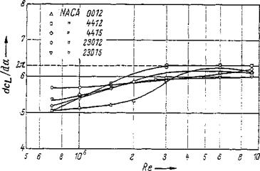
Lift slope For the profile NACA 2412, Fig. 2-39 gives the lift coefficient Ci against the angle of attack a from Jacobs and Sherman [29]. Figure 2-39a shows that for the range from Re= 8 • 104 to 3 • 106, no important effect of Reynolds number on the lift can be expected as long as the profile is not too much inclined (a < 8°). Since the cL{a) curve is linear in this a range, the Reynolds number influence can be described simply by the lift slope dci/da. This kind of presentation is used in Fig. 2-40 for a few four – and five-digit NACA profiles. These measurements show a slight increase of the lift slope dcL/da with the Reynolds number for Re < 3 • 106; beyond this Reynolds number, up to Re — 107, practically no change occurs.

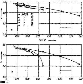
In addition, the lift slope depends on both the profile thickness and the trailing-edge angle. It decreases with increasing thickness ratio tfc in the four – and five-digit NACA profiles, whereas the opposite behavior is found in the NACA 6- series, namely, an increase of dc^Ida with increasing thickness ratio t/c.

Conversely, increasing the trailing-edge angle always results in a reduction of the lift slope. The quotient к = (dcLjda)expl(dcLlda)theoT is plotted in Fig. 241 as a function of the trailing-edge semiangle т (see Fig. 2-lb). The quotient x goes to 1 when the trailing-edge angle approaches zero (V = 0). When т increases, the quotient x declines to about 0.8 for smooth surfaces, and to 0.7 for rough surfaces (see also Hoemer and Borst [25]). The deviations of the measured lift slopes from the theoreti­cal values are caused by the boundary layer and the wake near the trailing edge.

The difference in boundary-layer thickness on the upper and the lower profile surfaces—thicker above, thinner below—is equivalent to an additional negative
camber; compare also Pinkerton [44]. The boundary layers change the Kutta condition, too, in that the rear stagnation point shifts from the trailing edge to the profile upper surface.

At extremely small profile Reynolds numbers, Re < 10s, such as occur in free-flight airplane models (see Schmitz [57]), often no linear relationship exists between lift coefficient cL and angle of attack a, even for very small angles of attack. In this case the measured cL values deviate strongly from theory over the whole angle-of-attack range, because the flow is widely separated from the profile. Conversely, at larger Reynolds numbers, Re > 10s, the separation that is caused by

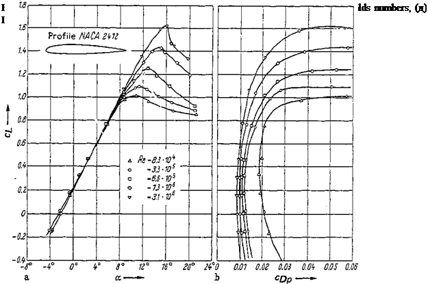Figure 2-40 Reynolds number in­fluence on lift slope dci/da for four – and five-digit NACA profiles with smooth surfaces.

Figure 2-41 Comparison of the lift slope from theory and experiment for NACA profiles of various trailing-edge angles 2r, where * = (rfc£,/ria)exp/ (cfc^/rfoOtheor – (fl) Smooth surface, (b) Rough surface.

a steep pressure rise on the suction side of the profile occurs only at larger angles of incidence, a= 5-20°, depending on the profile shape. The lower value of a is valid for thin profiles. As soon as local separation occurs on the wing, the lift slope decreases. The deviation from the linear characteristic of the theory grows larger with an extention of the range of separated flow on the profile until finally, at large a, the flow is almost entirely separated on the suction side, and the lift drops, as demonstrated in Fig. 2-116. The phenomenon of separation from the wing, which is to be discussed later in detail, has a decisive effect on the maximum lift coefficient CL max • This coefficient is of great aeronautical importance (in take-off and landing).

Maximum lift The aerodynamic problems of maximum lift are summarized by, among others, Nonweiler [43], Schlichting [54], and Smith [60]. The maximum lift of a profile depends decisively on the flow conditions in the boundary layer on the suction side. At very small Reynolds numbers, the boundary layer is completely laminar and separation occurs near the profile nose (leading-edge stall) because of the strong pressure rise on the suction side immediately downstream of the leading edge. The location of the separation point is almost independent of the Reynolds number. The maximum lift is, therefore, independent of the Reynolds number in this range. Only at a certain larger Reynolds number, the value of which depends on the profile geometry, do the flow characteristics change. The laminar boundary layer still separates; transition to turbulent flow now takes place in the separated flow, however, leading, in general, to reattachment of the turbulent boundary layer farther downstream. In this way, a laminar separation bubble forms between the points of laminar separation and turbulent reattachment. The reattachment point moves upstream with increasing Reynolds number until it finally reaches the separation point, that is, until the length of the separation bubble becomes zero. The maximum lift increases strongly with Reynolds number as a result of the
superposition of two effects: In the first place, lift is gained at a fixed angle of attack because of the reduction of the separation length, and then the wing can be set at a higher angle of attack before the flow ultimately separates.

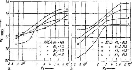
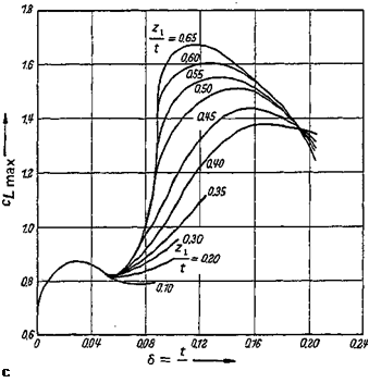
At very high Reynolds numbers, a natural transition from the laminar to the turbulent boundary layer occurs before the point of laminar separation. This transition point travels upstream with increasing Reynolds number and the length of the turbulent boundary layer, and consequently the boundary-layer thickness increases. As a result of this process, the circulation around the profile is diminished; that is, the maximum lift may again decrease somewhat at high Reynolds numbers. As an example for the cirnax behavior, the maximum lift of profiles of the NACA 6-series is plotted in Fig. 2-42 against Reynolds number for various thickness ratios t/c and camber heights hjc according to Loftin and Smith [29]; see also Fig. 2-39. In the range Re> 106 of interest to aeronautics, profiles of moderate thickness (t/c ~ 0.12) produce the largest lift. The influence of camber is reflected in an increase of cLmax with hjc because the critical, separation promoting pressure rise on the profile suction side is occurring at larger angles of attack for increased h/c. The most important geometric parameter affecting separation at large angles of attack, and thus affecting the maximum lift, is the shape of the profile nose, because this shape determines decisively the pressure distribution in the vicinity of the leading edge. The measurements by Nonweiler [43] of Fig. 2-43 convey some insight into these relationships through curves that show с^г max values for a fixed Reynolds number (Re = 6 * 106) as a function of the thickness ratio t/c. The nose radius is characterized by the profile ordinate zx at x = 0.05c. Accordingly, the nose radius has no effect on C£raax for very thin profiles, whereas for profiles of moderate thickness, cLmax increases considerably with zv It.

A similar parameter, namely, the ordinate z0/c of the profile suction side at station x/c — 0.0125, has been used by Gault [77]. It allows delineation of ranges of the various separation processes as a function of Reynolds number in a universal diagram. This presentation, Fig. 2-44, is based on measurements on about 150

Figure 242 Maximum lift coefficient of profiles of the NAC’A б-series vs. Reynolds number, (a) Effect of thickness ratio. (b) Effect of camber ratio.

Figure 2-43 Maximum lift coefficient at Reynolds number Re = 6 • 106 vs. thickness ratio t/c and nose radius in terms of zl/t. zx=z (x/c = 0.05). After [43],

profiles with smooth surfaces at low wind-tunnel turbulence. It shows that profiles with sharp leading edges, or with very small nose radii (z0/c < 0.009), have, at all Reynolds numbers, a specific separation characteristic that is termed thin-airfoil stall. Even at small angles of attack a, separation of the flow over the thin leading edge occurs directly at the profile nose, followed by reattachment. The velocity profile of the boundary layer at the point of reattachment is neither typically laminar nor typically turbulent. Not before the boundary layer approaches the trailing edge is a fully turbulent flow pattern established (see McCullough and Gault [77]). Reattachment occurs more and more downstream when the angle of attack increases, leading to a growing separation range and consequently a gradually diminishing lift slope. As soon as the flow is detached on the whole suction side, cL decreases continuously with increasing a (see also Young and Squire [77]).

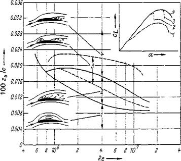Figure 2-44 Separation from profiles vs. Reynolds number and nose radius [in terms of z0/c, with z0 = z (x/c = 0.0125)], after [77]. (1) Separation from a thin profile. (2) Laminar separation from profile nose. (3) Combination of laminar and turbu­lent separation. (4) Turbulent separa­tion.

A basically different separation characteristic is found on wings of moderate thickness having a moderately large nose radius, the leading-edge curvature of which is, however, still relatively large.[10] The steep pressure rise behind the profile nose then leads to separation of the laminar boundary layer at larger angles of attack. The transition to turbulent flow takes place, however, in the separated flow that results in reattachment farther downstream. A laminar separation bubble is formed, the extent of which decreases with increasing angle of attack because the transition point, and with it the turbulent reattachment point, move closer to the separation point, which moves likewise toward the leading edge. Eventually, the laminar boundary layer separates on the very nose where the contour curvature is too large for the transition to cause reattachment. This process, known as the leading-edge stall, is characterized by a sudden sharp lift drop (see Crabtree [11] and Tani [64]).

On the other hand, on most thick profiles (f/c>0.15), that is, at large nose radii, flow reattachment occurs behind the laminar separation point, even at large angles of attack. In this case the maximum lift is determined by two processes that influence each other. These are the expansion of the laminar separation bubble from the nose, and the turbulent separation that starts at the trading edge and moves upstream with increasing angle of attack (combined leading-edge and trailing-edge stall). The variation of the lift ci{a) depends on the predominance of one or the other of these two separation processes. The separation bubble may disappear entirely on very thick, strongly cambered profiles and at very high Reynolds numbers. The reason for this is that the Reynolds number is then large enough for a natural transition to turbulent flow upstream of the station of strong pressure rise. The turbulent boundary layer separates only a short distance upstream of the trailing edge (trailing-edge stall). This separation point moves upstream continuously with growing angle of attack, and the lift does not drop abruptly after passing Cl max hut very gradually, similarly to the case of the thin profile. The profile shape of optimum lift coefficient at flow without separation can be computed following a procedure of Liebeck [38].

Pressure distribution In Fig. 245, pressure distributions on profiles of the NACA 6- series are presented in the range of the maximum lift at a Reynolds number Re = 5.8 * 106 according to McCullough and Gault [77]. Separation from thin profiles (NACA 64A006) is characterized by a very slight underpressure near the leading edge. This underpressure is even reduced with an a increase, whereas the separation range (cp = const) grows from the profile nose downstream. Conversely, a very strong suction peak exists on profiles of larger thickness ratio for a <<4?£max- ^he laminar separation bubble is too short to be noticeable in the pressure distribution, if it exists at all. The NACA 63i-012 profile causes laminar separation at the nose, resulting in an abrupt collapse of the high underpressure on

Figure 2-45 Measured pressure distribution at Reynolds number Re — 5.8 • 10e on profiles of NACA 6-series with various separation character­istics in the range of maximum lift. (1) Separation from thin profile. (2) Laminar separation from profile nose. (3) Turbulent separation.

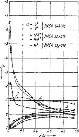the leading edge and an immediate flow separation over the entire suction side. This in turn results in the steep lift drop when the angle of attack for Cjr, max is exceeded. As soon as turbulent separation has been established, as is the case on the NACA 6З3-ОІ8 profile, the suction peak at the leading edge remains, even when a is larger than aCLmax- The separated range expands from the trading edge farther and farther upstream, causing the lift to decrease continuously.

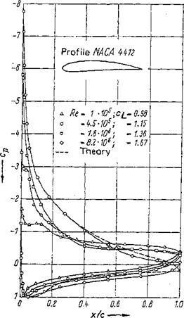
The separation characteristics of a given profile may be different for the various Reynolds numbers, as shown in Fig. 246 for the example of the pressure distribution on the profile NACA 4412 at the angle of attack a = 16° (see Pinkerton [29]). For Re = 1 • 10s and 4.5 • 10s, the pressure distribution is similar to that of the profile NACA 64A006 (Fig. 245); that is, separation has the same character on thin profiles, although only at larger angles of attack. The separated range decreases with increasing Reynolds number in this case. According to Fig. 244, for the thin profile at Re< 106, there are only two possibilities, namely, laminar separation or turbulent separation near the trailing edge. Transition from one behavior to the other requires that the profile is made thicker when the Reynolds number is reduced. When the Reynolds number is raised to 1.8 • 106, a laminar separation bubble 0.005c long forms on the NACA 4412 profile, and at x/c = 0A0 turbulent separation sets in. Finally, at Re = 8.2* 106, the flow is attached over the whole profile. A further increase in Reynolds number has practically no influence on the pressure distribution, which agrees quite well with theory as long as no separation occurs (see Cooke and Brebner [10]). Note,

Figure 2-46 Effect of Reynolds number on pres­sure distribution on profile NA. CA 4412 at a large angle of attack (a= 16°).

however, that the theoretical curve of Fig. 2-46 is obtained from a modified theory from Pinkerton [44] and not from pure potential theory.

The influence of the boundary layer on the pressure distribution on a profile as a function of angle of attack is presented in Fig. 2-47. Figure 2-47д gives the distribution at moderate angles, which is susceptible of computation after the

methods of potential theory. At larger angles of attack, separation sets in first on the upper surface of the profile near the trailing edge (Fig. 247b). From there, it travels upstream with increasing angle of attack. At the same time a wake forms in which a vortex (bubble) is embedded. At very large angles of attack, beyond the maximum of the lift coefficient, the wake shifts upstream to the wing nose (Fig. 247c). The flow reattaches again further downstream.

A comprehensive listing of experimental data on the lift problem is found in Hoerner and Borst [25].

Based on studies of Preston [61], Spence [61] makes some recommendations about the theoretical inclusion of the friction effect into the aerodynamics of the wing profile. Theoretical determination of the pressure distribution for separated incompressible flow about profiles of almost any shape is possible using a computational method of Jacob [27], but the abrupt leading edge separation and reattachment of the flow cannot be obtained directly by this method.

Airfoil in curved flow So far, it had been assumed in all considerations of profile theory that the wing moves in straight incident flow. When investigating the interference of the airplane parts with each other, the case is encountered, however, where the wing lies in a curved incident flow field. The aerodynamic problems of such a wing can also be treated with the skeleton theory.

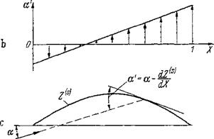
A flat plate in curved flow behaves approximately as a cambered skeleton in parallel flow. The variable angles of attack a(X) along a profile in curved flow can be replaced by changed equivalent skeleton line inclinations (a— dZ^jdX), as shown in Fig. 2-36. With this procedure in mind,

= a —d{X)

must be substituted in the formulas of the skeleton theory (Sec. 24*2). By using the expressions of Table 2-1, the mean angle of attack a is obtained as

71

a = ~ j’^(f) (1 + oos<p)d<p (2-112fl)

о

This is, to express it again in a somewhat different way, the angle of attack that produces in straight flow the same lift cL = 27ra as the variable angle-of-attack distribution. The zero-moment coefficient becomes then

cj/o— —J/ «'(<p) (eosip-f cos2<p) dy (2-1126)

0

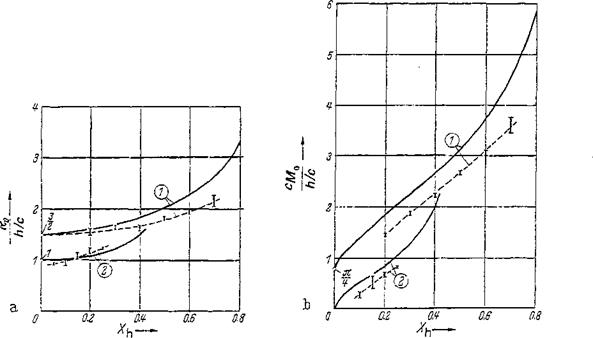
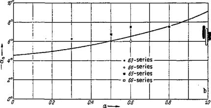
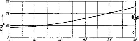
At a constant angle-of-attack distribution oc(X) = a, the above equations produce the relationships for the inclined plate: a = a, c^o — 0. Approximate expressions for a and cM0 have been derived by Pistolesi [45] and Multhopp (see Chap. 5 [40]), respectively. Using only local a values on a few characteristic stations of the chord, they arrived at the expressions

5 = OC.7S (2-113fl)

L

a’

Figure 2-36 Airfoil in curved flow-sche­matic explanation, (л) Variation of a on plate. (b) Angle of incidence distribution a'(x). (c) Skeleton profile Z^s

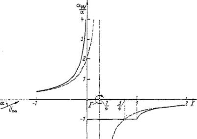
Figure 2-37 Distribution of the induced downwash angle on the extended wing chord for the inclined flat plate.

C. V0 = (aoo ~b 2a50 — Зато) (2-1 ЪЬ)

where ol’qo, a5Q, a’7S, and a’10O mean the local angles of attack a at the stations X= 0, 0.5, 0.75, and 1.0, respectively. Hence, the value of the angle of incidence at the 4-chord station should determine the lift when the angle-of-incidence distribu­tion is variable. Compare the formulas of Weissinger [73].

Theorem of Pistolesi The two approximation formulas of Pistol’esi and Multhopp are of particular importance when the continuously distributed circulation on the wing chord is replaced by a single vortex at the | – chord station, as is customary for simplified treatment of the wing of finite span (lifting-line theory, Sec. 3-3-4). The Pistolesi approximation for the mean angle of incidence is in agreement with the exact solution, as seen in Fig. 2-37. The Multhopp approximation for the zero moment produces the right value cMQ = 0 for the flat plate, because a[ю = —a50 and o4o = 3a’ltw when the plate is replaced by a single vortex at the | -chord station.

The velocity near-field of the profile So far, the velocity distributions have always been determined on the profile surface. For certain aerodynamic problems of airplanes, for example, for investigations into the influence of the wing on the incident flow of the fuselage or horizontal stabilizer, knowledge of the velocity field off the wing is required. This matter will now be discussed to some extent.

First, let the wing be replaced by its skeleton profile; that is, it is represented by its vortex distribution, Eq. (2-44). Of main interest are the z components w of the velocities because they produce a change of the effective angles of incidence on the airplane components that lie before and behind the wing. The induced velocity component w will be considered only in the wing plane, that is, on the ;c axis.

The distributions of the induced upwash and downwash velocities along the л axis are given by Eq. (246b):

і

mW=-T^I-T=lFdX’ (2-! 14)

o

Here k(x) is the circulation distribution along the profile chord and X=x/c, the dimensionless coordinate in direction of the profile chord. The total circulation of the wing Г is found from the circulation distribution by integration [see Eq. (2-52)]. Evaluation of Eq. (2-114) over the profile chord, 1, was described

earlier using the Birnbaum-Glauert substitution for the circulation distribution [Eqs. (2-61) and (2-63)].

Equation (2-114) can also be used to compute the induced downwash velocity before and behind the profile. A singular point of the integrand no longer exists in this case, however. The previous substitution of Eq. (2-62) now must be replaced by

X= £(1 ±cosh<y) (2-115a)

= + eosy’) (2-115b)

The lower sign applies to points before the wing and the upper sign to those behind the wing. By introducing Eqs. (2-115) and (2-61) into Eq. (2-114) and integrating, the downwash angle distribution aw = w/Uoo is obtained as

for X> andXCO[9]

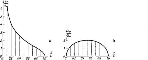
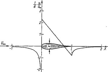
In the circulation distribution Eq. (2-61), the term with A0 represents the flat plate inclined by the angle a, with A0 = a. The term with A1 represents the parabola skeleton with camber h/c in a flow parallel to the chord with A v =4h/c. For the first case, the distribution of the downwash angles along the profile chord is plotted in Fig. 2-37. For comparison is shown the induced downwash angle distribution that is obtained when the wing is substituted by a single vortex of total circulation Г, located in the center of action XA of the distributed circulation, that is, at XA = of the inclined plate. At large distances before and behind the wing, the distributions of the induced downwash angles of the continuous vortex distribution (lifting wing) and the single vortex (lifting line) are in agreement.

It is noteworthy that in the case of the inclined plate, the induced downwash velocities at station X = f are equal for the lifting surface and for the lifting line (Pistolesi theorem).

In the case of flow around thick profiles, the main interest is directed toward the induced velocity и in the x direction before and behind the profile. From Eq.

Figure 2-38 Distribution of in­duced longitudinal velocity on the extended wing chord for a sym­metric Joukowsky profile (5 = t/c = thickness ratio).

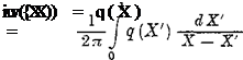
(2-91 a), this component is obtained by introducing the source distribution from Eq. (2-102). The evaluation is analogous to that of w(x) and produces for u(x)/U„ an equation analogous to Eq. (2-116), where the coefficients An of the circulation distribution must be replaced by ~Bn of the source distribution. The latter satisfy the closure condition Eq. (2-103). In Fig. 2-38, evaluation of such a computation is shown for a symmetric Joukowsky profile.

Although it is not possible in this book to cover the problems of unsteady flow that are of importance to airplane aerodynamics, the fundamental study of Wagner [72] on unsteady wing lift in plane flow should not be overlooked.

Computation of the velocity distribution on the profile contour The general case of a cambered profile of finite thickness will now be treated, after the case of the very thin profile (skeleton) discussed in Sec. 2-4-2 and the case of the symmetric profile of finite thickness in chord-parallel flow discussed in Sec. 24-3. The general case is obtained essentially by superposition of these two previously discussed cases.

A cambered profile of finite thickness can be composed of a skeleton line Z(s) = z^/c and a teardrop profile Z^ — z^jc (Fig. 2-1). In Eq. (2-1), the profile ordinates are given as

zUil = z^±zW

where the upper sign is valid on the upper surface, the lower sign on the lower surface. With Zu, the ordinates on the upper surface, and Zh those on the lower surface, Eq. (2-108) can be broken down into

^ = I (Zu + Z,) and z<*> = І (Zu – Zi)

The velocity distribution of the general profile is the sum of those of skeleton and teardrop. A third distribution has to be added, however, which is produced through the inclination of the teardrop profile. Riegels [49] computed this contribution. The velocity contribution caused by the inclination of the teardrop profile may be interpreted as the influence of an additional camber and an

1(1-Z) (*Щ

additional angle of attack, as was shown in [68]. Accordingly, the following contributions have to be added to the geometric skeleton (mean camber) line Z^:

^ = -2“(^).V-0 (2’U№)

The equations for the computation of velocity distribution and aerodynamic coefficients that were derived by the method of singularities in the cases of skeleton and teardrop profiles can be evaluated conveniently through numerical quadrature formulas. Details for the computations are found in [49].

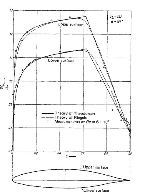
The result of a sample computation from the above outlined method for the computation of velocity distributions on profiles is presented in Fig. 2-35 for the profile NACA 66 (215)-216, a — 0.6. A theoretical velocity distribution from Theodorsen and Garrick [66] (conformal mapping) is also shown, and for comparison with the theory, a measurement from [1] is added. The agreement of the two theoretical curves with the test data is good. Note the appreciable agreement of these pressure distributions for the inclined symmetric Joukowsky profile, obtained by the method of singularities, with those of Fig. 2-16, computed by the method of conformal mapping.

Lift and pitching moment The computation of the aerodynamic coefficients for the skeleton profile was discussed in Sec. 24-2. The results in that section are also valid for the inclined profile of finite thickness if the influence that is introduced by the inclination of the teardrop profile in Eq. (2-110) is taken into account. The resulting relationships for lift slope and neutral-point location are given in Table 2-1.

The other aerodynamic coefficients (zero-lift angle of attack, zero-moment coefficient, angle of attack, and lift coefficient of the smooth leading-edge flow) are equal for the profile of finite thickness and the skeleton profile.

For the Joukowsky profile in Eq. (2-100) the lift slope is

………………………………….. – 2rr(l………….. – b e) = .2zt(l – 0.77 <5)………. _ . (2-11 la)

da

(24Ш)

in agreement with the solution from the method of conformal mapping, Eq. (2-33).

For the NACA profiles of Fig. 2-2, these formulas show that the lift slope always increases with thickness, whereas the neutral point lies behind the c/4 station of the profile. The test data of the lift slope from [1] lie in all cases below the theoretical values. When the profile thickness increases, the lift slope of the older NACA 00-series with a relatively large trailing-edge angle decrease’s (Fig. 2-2b), whereas it shows the theoretical trend in the newer NACA 6-series with a smaller trading-edge angle (Fig. 2-2c). In ah cases, the lift slope is smaller when the surface

Figure 2-35 Velocity distribution on the profile contour of profile NACA 66 (215)-216, a — 0.6. Lift coefficient c£ = 0.23. Comparison of theory and experiment.

is rough than when it is smooth. This behavior shah be taken up again in Sec. 2-5. A similar comparison shows disagreement of measurement and theory for the neutral-point location of the older NACA series.

Using a procedure by Martensen [28], Jacob [28] extends the singularities method by arranging vortices on the profile contour instead of the profile chord. The investigation of Lan [37] and the comments by Maskew and Woodward [40] should be mentioned. Furthermore, profile theories of higher order for incom­pressible flow are found in, among others, Keune [22, 32] and Lighthill [39]. An – essential contribution to the theoretical and experimental investigations of fluid mechanical behavior behind blunt profiles has been made by Tanner [65]. Base pressure and base drag play an important role in this case.

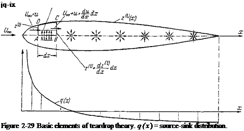
Fundamentals of teardrop theory The term teardrop profile means a symmetric profile of finite thickness. With the method of singularities, a teardrop profile is obtained through superposition of a source-sink distribution along the profile chord with a translational flow (Fig. 2-29). Let a continuous source-sink distribution be given along the profile chord, the source strength per unit length of which is q(x). This source distribution induces the velocity component u{x) in the x direction and produces the velocity component w(x) in the z direction (Fig. 2-29). Let z^(x) be the equation of the upper surface of the teardrop with the coordinate origin on the

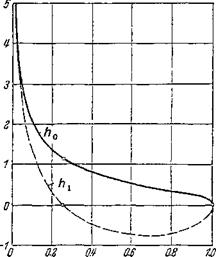Figure 2-27 The functions h0 and hx for the pressure distribution on the chord at given lift and moment coefficients [Eqs. (2-87) and (2-88) j.

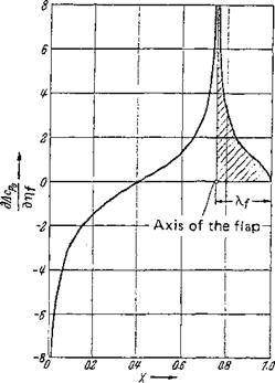
Figure 2-28 Theoretical pressure distribution of the folded plate (flap wing) of Fig. 2-24 at zero lift [Eq. (2-89)]. Chord ratio of flap and wing Лf=cf/c = 0.25.

leading edge. Then, the relation between source distribution and teardrop shape is obtained easily by applying the continuity equation to the area element ABCD in Fig. 2-29, with the result

{U oo + u) 2^ + -2"?^a;=|^co – f-tt-j – [%№ – j

From this the source distribution in linear approximation is obtained as

= 2^[(t7O0+и)гй] C2-90 a)

= 2 (2-90 b)

For teardrops of moderate thickness, the induced velocities и can be disregarded as compared with £/», with the exception of the vicinity of the stagnation point.

In the case of thin profiles it can be assumed that the velocity components on the teardrop contour are approximately equal to the values on the profile chord. In analogy to Eq. (246), the components of the induced velocity on the chord are obtained as

To obtain a closed profile contour, the total strength of the source-sink distribution must be zero (closure condition):

c

J q(x) dx = 0 (2-92)

.! = 0

In computing the source-sink distribution for a given teardrop shape z^x), the closure condition is automatically fulfilled because of Eq. (2-90).

With the profile chord length c, the dimensionless quantities

y r(r)

X=f and Z<f) = ^ (2-93)

will now be introduced.

The kinematic flow condition, namely, that the profile contour is a streamline, is

dzU) w(x)

dx £7 со

It can be verified immediately that this condition is identical to Eq. (2-90b).

According to Riegels [49], the velocity distribution on the contour is then established by division with

(2-95)

Here, 1/х(х) is called the Riegels factor. Since l/x(x) is zero at the leading edge, it is assured that the velocity goes to zero at the front stagnation point, and the velocity distribution on the contour is finally

T-FC(X) _ 1 / 1 г dZ<l) dX’

t/oo *(Z) + nj dX’ X-X’

In this way, the computation of the velocity distribution for a given teardrop profile has been reduced to a quadrature formula.

By disregarding the Riegels factor, the velocity distribution on a simple biconvex parabola profile becomes

Here, 5 is the thickness ratio t/c. The highest velocity occurs at X = with the value UjniJUoo = (4/я)6. Likewise, the velocity distributions for the extended parabola profiles from Eq. (2-6) can be computed (see Truckenbrodt [49]).

For the evaluation of the quadrature formula, Riegels [49] introduces the Fourier series

Z(0 = sinv 99 X = |(1 + COS99) (2-98)

V ш 1

Wc(<p) _ 1 Uoo [8]W)

in analogy to Eq. (2-85). When this expression for is inserted into Eq. (2-96), the velocity distribution on the contour assumes the simple form

The numerical evaluation of the equation by means of simple quadrature formulas is treated in [49].

From Eq. (242), the contour of the thin symmetric Joukowsky profile* is given by

Z(r) = sin v>(l — cos ф) (2-100a)

= 2e^X(l-X)3 (2-100 b)

where

At 1

£=——4 = 0.775 and xf=4 ЗуТ c f 4

The Fourier coefficients are bt = £, b2 – —ejl, and h3 = b4 = ■ • • = 0. Consequently, the velocity distribution on the contour is given by

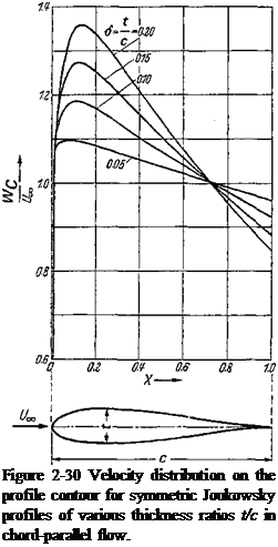
Figure 2-30 shows the velocity distributions computed by Eq. (2-101) for various thickness ratios. Within the accuracy of the plot, complete agreement of the approximate and the exact solutions by conformal mapping is obtained. See Fig.

2- 16 for cL = 0. Because the trailing-edge angle of the Joukowsky profiles is zero, the velocity distribution has no rear stagnation point on the trailing edge.

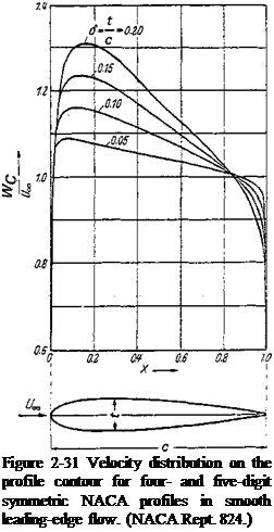
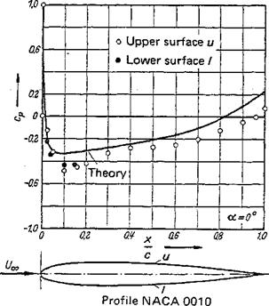
For the four – and five-digit NACA profiles from Fig. 2-2a, the theoretical velocity distributions may be found in [1]. A few distributions at various thickness ratios 5 = t/c are shown in Fig. 2-31. They were computed by the procedure of Theodorsen and Garrick [66]. Values computed by the singularities method deviate only slightly from them. The teardrop shapes of the NACA 6-series, Fig. 2-2c, were established from given velocity distributions, which were determined mainly by the location of the maximum velocity. In Fig. 2-32, the velocity distributions are shown for the four profiles of Fig. 2-33 with a thickness ratio 5 =0.12. Figure 2-33 gives a comparison between theoretical and experimental pressure distributions on the NACA profile NACA 0010 and shows good agreement.

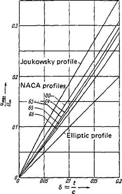
The maximum velocity on a profile is of considerable importance for the

behavior of the profile at high subsonic velocities (critical Mach number. Sec. 4-3-2). In Fig. 2-34, the ratio of the maximum velocity difference to the constant translational velocity is given against the thickness ratio of most of the teardrop profiles discussed above. Accordingly, the maximum velocity depends heavily on the thickness distribution for an otherwise unchanged thickness ratio. The elliptic profile produces the smallest velocity difference, the Joukowsky profile the largest.

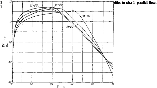Figure 2-33 Comparison of theoretical and experimental pressure distributions for the symmetric profile NACA 0010 in chord – parallel flow.

Figure 2-34 Maximum perturbation velocity wmax of teardrop profiles in chord-parallel flow vs. thickness ratio 5 = t/c.

Computation of the teardrop profile from a given velocity distribution In analogy to the Birnbaum-Glauert series expansion for the distribution of circulation in the case of skeleton theory [Eq. (2-61)], the source distribution will now be represented in the form of a trigonometric series (see, e. g,, Allen [3] ):

q(<p) = 2 Uoo (b0 tan-— – f Z Вя si™ yj j (2-102)

The relation between x and <p is given in Eq. (2-62). The closure condition for the profile contour, Eq. (2-92), is satisfied when

2B0 +Bi = 0 (2-103)

By introducing Eq. (2-102) into Eq. (2-9Ід), the induced velocity in the x direction is obtained as

The profile contour is determined by introducing Eq. (2-102) into Eq. (2-90b) and integrating along X:

The first term represents the Joukowsky profile, as can be verified by comparison with Eq. (2-100). Profile shape and velocity distribution are interrelated by Eq. (2-96), which must now be interpreted as the integral equation for the profile inclination dZ^/dX. Following Betz [4] and Fuchs [16], the solution is

where

denotes the induced velocity distribution on the chord, and % is defined in Eq. (2-95). Since the needed profile inclination is a term of this equation, Eq. (2-106) can be solved only through iterations (see Truckenbrodt [68]). The publications by Eppler [13] and Strand [63] on this subject should also be mentioned.

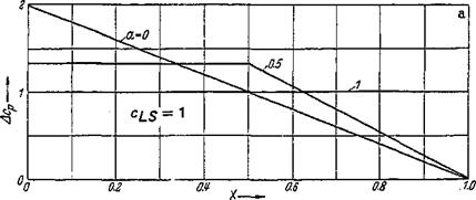
The simplest case of a constant induced velocity и on the chord leads to an elliptic teardrop profile. For a linear distribution of the induced velocity и/иж,

/- = <5(1 – bX)

u oo

the profile contour takes the shape

Zw = [4 – 6(1 + 2X)-]VX{1 – X)

For b = 0 the profile is elliptic; for b — f, the Joukowsky profile [Eq. (2-100)] is obtained.

Fundamentals of skeleton theory As was stated above, the very thin profile (skeleton profile) is obtained by superposition of a translational flow with that of a distribution of plane potential vortices. This theory has therefore been termed the theory of the lifting vortex sheet. It was first developed by Birnbaum and Ackermann [8] and by Glauert [17], and later expanded in several treatises, particularly by Helmbold and Keune [22, 32], Allen [3], and Riegels [49].

For the following discussion a coordinate system as shown in Fig. 2-20a is used. Accordingly, the profile chord coincides with the x axis. The coordinate system origin lies on the profile leading edge. The mean camber line is given by z^{x). From Fig. 2-20a, the mean camber line is seen to be covered with a continuous vortex distribution. With the assumption that the skeleton profile has only a slight camber and, therefore, rises only a little above the profile chord (x axis), the vortex distribution can be arranged on the chord instead of the mean camber line (Fig.

2- 20b). The mathematical treatment of the problem is considerably simplified in this way.

The vortex strength of a strip of width dx of the vortex sheet is, from Fig.

2- 20 b,

Неге, к is the vortex density (vortex strength per unit length) or the circulation distribution. By applying the law of Biot-Savart, the velocity components in the x and z directions, respectively, that are induced by the vortex distribution at station x, z are

C “t[7]’2)- 2* (х-*)> + г‘ ІХ’ 0 (245a) C 10 {x, *) — 2jr jk (X ) ^ _J_ г2 dx (245b) О

For slightly cambered profiles, the velocity components on the skeleton line are approximately equal to the values on the profile chord (z = 0). The velocity components on the chord are obtained through limit operations as z -> 0 of Eqs. (245a) and (2456)

were introduced in Sec. 2-1, with c being the chord length.

The velocity component и is proportional to the vortex density. The upper sign is valid for the profile upper surface, the lower sign for the lower surface. When crossing the vortex sheet, the velocity component и changes abruptly by an amount

Au — uu—Ui — k (248)

The integral for the velocity component w has a singularity at X’ = X*

The distribution of the vortex density on the chord is determined by the kinematic flow condition, which requires that the skeleton line is a streamline. Specifically, a translational velocity Ux is superimposed on the vortex distribution that forms the angle of attack a with the chord (Fig. 2-20).

The kinematic flow condition can also be formulated by the requirement that the velocity components normal to the mean camber line must disappear. Within the framework of the above approximation, it is sufficient to satisfy this condition on the chord instead of the mean camber line, resulting in

	(249)

This equation relates the angle of attack a and the ordinates of the camber to the induced normal velocities w.

The velocity distribution on the profile surface and the vortex density are related by

U(X)=U„ + u(X)**U„±lk(X) (2-50)

This relationship is valid for small angles of attack according to Eq. (246a).

The Kutta condition, Sec. 2-2-2, requires that the velocities on the profile upper and lower surfaces be equal at the trailing edge. It is required, therefore, that in Eq. (2-50),

k = 0 for X = 1 (2-51)

The total circulation around the profile is determined from the distribution of the vortex density as

Г= Jk(x) dx = c j’lc(X)dX

The pressure difference between the lower and upper surface is obtained by means of the Bernoulli equation:

Pi Pu Q Ifoo А Ы Q Uook

With Eq. (248), the dimensionless pressure coefficient takes the form

with q„ —qUlell being the dynamic pressure of the incident flow. Consequently, the distribution of the vortex density produces directly the load distribution over the profile chord. From Eq. (2-10), the lift coefficient = L/q„bc is expressed by

cL = / AcJX) dX

The latter relationship may also be found from the interrelation of lift and circulation after the Kutta-Joukowsky equation (2-15) for wTC = Ux. Equation (2-12) yields the pitching-moment coefficient relative to the profile leading edge, cM =M/qoabc1 (tail-heavy = positive):

(2-55 b)

0

Computation of the mean camber line from the distribution of circulation Deter­mining the shape of the mean camber line and the angle of attack from a given distribution of circulation k(X) requires two steps. First, from Eq. (246b), the distribution of the induced downwash velocity w(X) is obtained along the profile chord. Then, this distribution is introduced into the kinematic flow condition, Eq. (249), and the following expression for the shape of the mean camber line is obtained by integration over X:

These two steps may be combined into one equation by introducing Eq. (246b) into Eq. (2-56) and integrating over X. The angle of attack and the integration constant C are determined in such a way that the ordinates of the mean camber line disappear on the leading and trailing edges, resulting in

for the mean camber line and

(2-58)

for the angle of attack as measured from the chord.

In the case of a constant distribution of circulation along the profile chord, к — 2U«,C, Eqs. (2-57) and (2-58) yield, for the mean camber line and the angle of attack,

— ■. ZM(X) = – — [(1 – X) ln(l – X) + X lnX] with Л = 0 (2-59)

The maximum camber height is h/c = (In 2jn)C = 0.221C and lies at 50% chord. This mean camber line is found in NACA profiles of the 6-series (see Fig. 2-2c; a = 1.0). The lift coefficient is obtained from Eq. (2-54b) as

Following up on the investigations of Birnbaum and Ackermann, Glauert [17] proposed the following Fourier series expansion for the circulation distribution in the two-dimensional airfoil problem:

(2-61)

X = 1(1 – j – cos 9?)

so that on the leading edge X = 0 and = u, and on the trailing edge X = 1 and V? = 0. Each term in Eq. (2-61) satisfies the Kutta condition, Eq. (2-51).

By introducing the expression for the distribution of circulation, Eq. (2-61), into the equation for the induced downwash velocity, Eq. (2-46b), the simple relationship*

(2-63)

is found after integration.

The interrelation of the Fourier coefficients of Eq. (2-63), the shape of the mean camber line, and the angle of attack are obtained with the help of Eq. (249) as

With a given distribution of the circulation, this is a differential equation for the mean camber line Z^SX).

The first two terms in Eq. (2-61) represent particularly simple mean camber lines: The distribution of circulation of the first standard distribution becomes

The distribution к is shown in Fig. 2-21 a. The induced downwash velocity is determined from Eq. (2-63) to be wlU„ = —A0, leading to

Further, from the kinematic flow condition, Eq. (2-64), it follows that the profile inclination dZ^/dX must be constant. This is possible only when Z^ = 0, and, therefore,

(2-66)

It has thus been shown that the first normal distribution represents flow about the inclined flat plate.

The second normal distribution is given by

1c — A1 k[j = 2 Uco Аг sin= 4£/co Ах |/Х(І —X) (2-67)

/

Figure 2-21 The first and the second normal distributions; circulation distribution by Eq. (2-61). (a) The inclined flat plate. (b) The parabolic skeleton at zero angle of incidence.

This is an elliptic distribution (Fig. 2-21 b). The induced downwash velocity is obtained from Eq. (2-63) as

^ = — cos cp = — (2 2Г – 1)

C/oo

and with Eq. (2-56), the shape of the mean camber line is given by

zW=AtX(l – X) = 4jX(l – X) with a = 0 (2-68)

This is a parabolic mean camber line with camber height h/c = Ai/A0. The results obtained for the inclined flat plate and the parabolic camber without angle of attack agree with the exact solutions found by the method of conformal mapping for small angles of attack, Secs. 2-3-2 and 2-3-3, respectively.* In particular, the relationships for lift and pitching-moment coefficients are also valid.

Computation of the aerodynamic coefficients Equations will now be presented that allow one to compute the aerodynamic coefficients directly from a given mean camber line. The lift coefficient is obtained from Eq. (2-54Z?) after integration t with the help of Eqs. (2-61) and (2-62) for the distribution of circulation as

cL=7t(2A0+Al) (2-69)

In the same way, the pitching-moment coefficient relative to the leading edge is obtained from Eq. (2-55b) as

Cm — —^"(2-d. o 2A^ – j – A%) (2-70)

This equation was first presented by Munk [41].

*Note that %Sc — X — .

tin this process, most of the integrals over <p disappear as a result of the orthogonality conditions of the trigonometric functions.

The angle of attack for zero lift (cL =0) is obtained by setting 2A0 = —A1} and the zero-lift moment coefficient becomes cM0 =—(ir/4)(Ai+A2). Conse­quently, the pitching-moment coefficient can also be written as

1

CM – CMO

From Eq. (1-29), the neutral-point location is given by —dcM/dcL = xNjc. Consequently, the distance of the neutral point from the leading edge becomes

XN _ 1

c 4

which is independent of the shape of the mean camber line.

The Fourier coefficients are found through Fourier analysis:

71 n

1 Г dZ{s) 9 Г dZ{s)

A0=cx-—J ~jY~d(P An=-^J -jj-costt <pd(p (n> 1) (2-73)

о 0

The integrals can be transformed through integration by parts into terms in which the camber line coordinates replace the camber line inclination dZ^/dX. By introducing the coefficients A0 and Ax into Eq. (2-69), the relation

dcT

it=2* w

is obtained for the lift slope, independent of the camber line shape, and the lift coefficient from Eq. (1 -23) is

cl~ 2іт(а—а0) (2-75)

The equations for a0 and cM0 are given in Table 2-1.

On the profile leading edge, X = 0, that is, = nr, in general the vortex density and consequently the velocity are infinitely large (Eq. 2-61). There is an angle of attack, however, for which the velocity remains finite on the leading edge. In Sec. 2-3-3, the designation of angle of smooth leading-edge flow was introduced for this angle of attack. This angle as can be determined from Eq. (2-61) by setting A0 = 0. The expressions for as and for the lift coefficient for smooth leading-edge flow are also presented in Table 2-1.

If there is flow around the leading edge, the velocity is infinitely high, streaming either from below to above, or vice versa. The strong underpressures near the leading edge produce a force acting upstream on the leading edge, called suction force in Sec. 2-3-2. The suction force coefficient cs = S/q„bc can be expressed by

1

cs = – j!- f k{X) w(X) dX

V CO J

0

Introducing Eqs. (2-61) and (2-63) into this equation yields

c, s = 2 я A‘i

Table 2-1 Compilation of formulas for the aerodynamic coefficients of cambered profiles of finite thickness Lift slope dcL da l 2 f Z 2n 1 -|—— ———— dm 1 71 J Sin^) r j 2л(і + 2 ez^ Zero-lift angle «0 n 2 Г Zw n J 1 — cos <p (^ 0 N -1 2 E вт z<s> Neutral-point location •Lv c 1 / 2 Г 1 + 2008^- 2003 2, * 4 1 71 J Sill Cp T J t (і + Ц’с-z’,::) Zero moment см о f 2cos,>-cos2,, J 1 — cos q> 0 2 E D, n Z<’> " Hi Angle of incidence for smooth leading-edge flow as 71 2 Г cos m ч, / . „ Zl>)dtp n J sm^ T 0 N -1 2 І7 Z<*> ^ и* 4» Lift coefficient for smooth leading-edge flow CLS n r ZM 4 . 0 dtp J sin – (p T 0 JV-l 2 27 Z(-> иг /ti ‘ See correction in [50].

and with Ci of Eq. (2-69) and cLS =nA1,

cs = 2^(cl ~cls)2 (2-77)

Consequently, the suction force is zero for smooth leading-edge flow, but grows with the square of (cL — cLS).

For a given distribution of circulation k{X), the coefficient A0 in Eq. (2-61) is obtained by the limit operation

A0 = lim [kQOVX]

ZUac 0

In the integral formulas of Table 2-1 for the computation of the various coefficients, only the. distribution of the mean camber coordinates appear

besides certain trigonometric functions of ip. In addition, simple quadrature formulas are given for the numerical evaluation of the integrals. Accordingly, the profile coordinates Zm = Z(Xm), at the stations Xm are multiplied with once-for-all-computed coefficients, Fm, and the sums are then formed of these products (see

Table 2-2).

In Table 2-3 a few results are presented that can easily be verified. Case (a) refers to a uniformly cambered skeleton line from Eq. (2-6); case (b) refers to an asymmetrically cambered line from Eq. (2-5).

For the case of a simple parabolic mean camber (Xh = |), the numerical values are

ot0=-2^ cM0 = -7tj as = 0 cls=4ttj (2-78)

u L C-

The profiles with fixed aerodynamic centers according to the discussion in Sec.

1- 3-2 are obtained from the above skeleton family by setting смо = 0. From Table

2- 3, case (b), it follows immediately that b = — f. This camber line has an inflection point (S shape). The case b = 0 is again the simple parabola skeleton.

Table 2-2 Coefficients А, В, C, D, E, F for the computation of the aerodynamic coefficients of Table 2-1 forrV= 12 (after Riegels (49,50]) m Хщ Am Вщ с Вщ F 1 т 1 0.9830 0.6440 -4.8919 0.6864 -7.9370 -2.4032 15.6333 2 0.9330 0 0 0.1667 -0.2267 0 0 3 0.8536 0.2357 -0.5690 0.3333 -1.0790 -0.2357 2.0944 4 0.7500 0 0 0.2887 -0.1309 0 0 5 0.6294 0.1726 — 0.2249 0.2387 -0.4210 -0.0462 1.1224 a 0.5000 0 0 0.3333 0 0 0 r- І 0.3706 0.1726 -0.1324 0.0601 -0.1402 0.0462 1.1224 8 0.2500 0 0 0.2887 0.1309 0 0 9 0.1465 0.2357 -0.0976 -0.3333 0.0318 0.2357 2.0944 10 0.0670 0 0 0.1667 0.2267 0 0 11 0.0170 0.6439 — 0.0848 -1.8017 0.1197 2.4032 15.6333

Table 2-3 Aerodynamic coefficients of uniformly and asymmetrically cambered skeleton lines Coefficient (a) Skeleton from Eq. (2-6) (b) Skeleton from Eq. (2-5) Zero-lift angle a° h 1 c 1-Xh – | (4 + 3b) Zero-moment coefficient cMo n h xh0 – 2Xh) 2 c 1-Xh – ^*(8 + lb) Angle of incidence for S. L.E. F.* as 1 h 1 —2Xh 2 c xha-xh) 1 OO | b – El Lift coefficient for S. L.E. F.* CLS h 1 77 c xha – xh) a(2 + b) *Smooth leading-edge flow.

In the NACA systematic listing, various skeleton line shapes are used (see Sec.

2- 1).

Four-digit NACA profiles In Fig. 2-22, zero-lift angles of attack and zero moments are plotted versus the maximum camber height (crest) location. Test results [1] are also shown for comparison with theory. Because of the slight effect of profile thickness in the range of thickness ratios 0.06 < t/c < 0.15, a mean curve of experimental data is shown. The plotted bars represent three data points each for cambers h/c = 0.02, 0.04, and 0.06. The agreement of theory and experiment is

Figure 2-22 Zero-lift angle of attack a0 and zero-moment coefficient cjvf0 of NACA skeleton lines. Comparison of theory and experiment from NACA Repts. 460, 537, and 610. Curve 1, four-digit skeleton lines. Curve 2, five-digit skeleton lines.

satisfactory. As a result of friction, the deviations increase somewhat with a downstream shift of the camber crest.

Five-digit NACA profiles In Fig. 2-22, results for zero-lift angle and zero moment are presented for the skeleton lines without inflection points. Test results from [1] are also shown. The influence of the profile thickness is again negligibly small. The plotted test data are the results for values of c^s ~ 03, 0.45, 0.6, and 0.9. Agreement between theory and experiment is better than in the case of the four-digit NACA profiles.

NACA 6-profiles The skeleton lines of the NACA 6-series have been established from purely aerodynamic considerations. Preestablished are the resultants of the pressure distributions on the lower and on the upper profile surfaces (Fig. 2-23a). The corresponding skeleton lines are presented in Fig. 2-2c.

For the aerodynamic coefficients, the following expressions are established:

(2-796)

(2-79 c)

Zero-lift angles of attack and zero-moment coefficients for cLS = 1 are given in Fig. 2-23b and c versus the quantity a. These results are compared with test results of NACA Rept. 824 and show satisfactory agreement.

Bent plate (flap, wing, control surface) Another valuable application of the skeleton theory is found in the calculation of the aerodynamic coefficients of the flap wing. By replacing the flap wing by a skeleton line, the bent plate, Fig. 2-24, is obtained. This problem was attacked first by Glauert [18].

With the assumption of a small deflection angle r]f, the ordinates of the skeleton line ZW = Zf, relative to an imaginary chord connecting the leading edge with the trailing edge of the deflected flap, are

zf=Wvf

where f— Cf/c is the flap chord ratio (see Sec. 3-1-1).

Since the profile inclinations are constant within the ranges of Eq. (2-80), integrations for the determination of aerodynamic coefficients can easily be performed. It is expedient to introduce in addition the following relationship for the position of the station:

The change of the zero-lift angle with flap deflection is measured relative to the fixed portion of the profile (wing, stabilizer) rather than relative to the imaginary chord. The change of angle of attack (= change of the zero-lift angle with flap deflection) is then given by

= ~ ~ (sin Pf + Pf) = ~~ ~ (%А/0 ~ V) arcs^ri VV ) (2-82a)

a—— Figure 2-23 Aerodynamic coefficients for skeleton lines of the NACA 6-profiles at the lift coefficient of the smooth leading-edge flow Cjr^ =1.0. Comparison of theory [Eqs. (2-79a)~ (2-79c)] and experiment, after NACA Rept. 824. (a) Pressure distribution Acp; (b) Zero-lift angle a0. (c) Zero pitching-moment coefficient c^Q.

Figure 2-24 Coordinates used in the skeleton theory of airfoils with flaps.

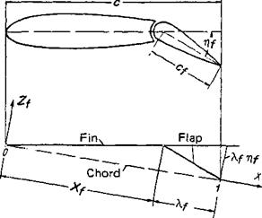The term da0/dr]f is frequently called the flap or control-surface efficiency, because it is a direct measure of the lift change caused by the flap (control surface). The flap efficiency vanishes for Xf = 0 and amounts to —1 for Xf= 1, that is, when the whole profile is being deflected as a flap.

The change of the zero-moment coefficient (moment change at constant lift) becomes

-g^jp = — у sin v?/( 1 + cos ^f) — — 2Vfy(l — X/)3 (2-82b)

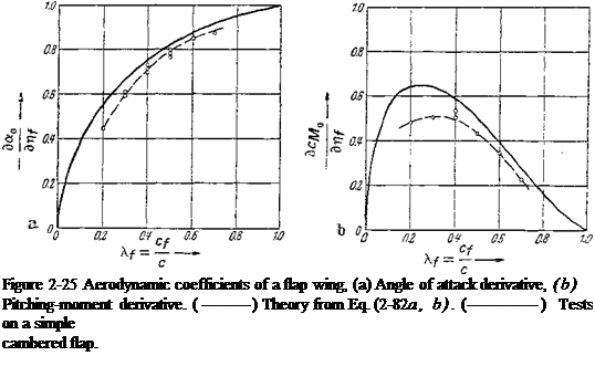
The results of the above formulas are shown in Fig. 2-25. The theoretical relationship between the aerodynamic flap coefficients and the flap chord ratios is well supported by measurements. In Fig. 2-25, the test results of simple cambered flaps by Gothert [21] are added. The deviations are again due to friction effects.

The aerodynamics of flaps and control surfaces will be discussed in more detail in Sec. 8-2-1.

Computation of the velocity distribution on the skeleton line The problem of computing the distribution of circulation and consequently the velocity distribution will now be treated for a given skeleton line shape at a given angle of attack. By introducing Eq. (249) into Eq. (2466), the equation defining the circulation distribution becomes

This is an integral equation for the vortex density к with given values of a — dZ^/dX. It was first solved by Betz [4]. By taking into account the Kutta condition Eq. (2-51) and Eq. (2-50), the velocity distribution about the skeleton profile (see also Fuchs [16]) is given by

For the case of the uncambered profile, = 0, the already known result for the inclined flat plate is valid; see Eq, (2-65). To evaluate the quadrature formula for the velocity distribution, Riegels [49] makes the Fourier substitution

ZW = Zavcosvcp (2-85 a)

V = 1

^ X = |(1 + coscp) (2-856)

Introducing these expressions into Eq. (2-84) makes elementary evaluation of the integrals possible.* The velocity distribution of the skeleton profile is then

where the upper sign is valid for the upper side, the lower sign for the lower side of the skeleton profile. Numerical evaluation of this equation by means of simple quadrature formulas is treated in [49] (see also [28]). The first term of Eq. (2-86) represents the velocity distribution of the inclined flat plate. For the parabolic skeleton

2(5) – — sin2 = t! r — (1 — cos 2ф) c 2 c

[see Eq. (2-68)], = hjc, a% = ~hjc, аъ = a4 = • • ■ = 0. Therefore, Eq. (2-86) yields,

for a = 0,

cos293 — 1 . , . h.

—– – I—— = 1 ^ 4— sing?

smg? c

a result already obtained in Eq. (2-67), taking into account Eq. (2-50).

Velocity and pressure distributions for the skeleton lines of the four – and five-digit NACA profiles, Figs. 2-2a and 2-2b, are given in [1]. In Fig. 2-26 some pressure distributions are presented for the angle of smooth leading-edge flow. For the skeleton lines of the NACA 6-series, pressure distributions have been presented in Fig. 2-23a.

Pressure distribution for given lift coefficient and moment coefficient The problem of approximating a given skeleton line by superposition of an inclined flat plate and a parabolic skeleton in such a way that lift and zero-moment coefficients of approximation and given skeleton are equal can be solved with the help of the above-introduced Fourier series expansion. In this case the Fourier coefficients from Eqs. (2-69) and (2-70) become

12 4

A° = 2wCl + n См° аПС^ =

Figure 2-26 Theoretical pressure distribution of NACA skeleton lines from NACA Rept. 824 at smooth leading-edge flow, (a) Four-digit NACA profile with h/c — 1.0. (b) Five-digit NACA profile with ci$ = 1.0.

These coefficients are introduced into Eq. (2-61), and the resultant distribution, taking into account Eq. (2-53), is obtained as	pressure
	A cp(X) = cLhQ (X) + см о 4h j (X)	(2-87)
with	MX) = !jand MX)=J-(l-4Z)j/!^	(2-88)

The distributions h0(X) and hl(X) are shown in Fig. 2-27.

Bent plate (flap wing) Finally, the pressure distribution of the bent flat plate (flap wing) will be mentioned. For the zero-lift angle of attack, cL = 0, the result is

In Fig. 2-28, the pressure distribution according to this equation is presented for the flap chord ratio Xf = . The cross-hatched area represents the load on the flap, the determination of which as well as that of the flap moment (control-surface moment) will be discussed in Sec. 8-2-1.