Our heavyweight helicopter equal in the world does not have
In Rostov started production of the most load-lifting rotary-wing car The Russian holding «Helicopt[...]

Everything about aircrafts and helicopters. News and events in aviation worldwide. Civil, transportation, military helicopters and airplanes.

Everything about aircrafts and helicopters. News and events in aviation worldwide. Civil, transportation, military helicopters and airplanes.

Everything about aircrafts and helicopters. News and events in aviation worldwide. Civil, transportation, military helicopters and airplanes.

Everything about aircrafts and helicopters. News and events in aviation worldwide. Civil, transportation, military helicopters and airplanes.


As an illustration, consider the hummingbird wing shown in Figure 3.5a. A major research interest is to probe the coupled dynamics between the fluid flow and the flexible wing. The fluid flow creates pressure and viscous stresses, which cause the wing to deform. The wing, in turn, affects the fluid flow structure via the shape change, resulting in a moving boundary problem [417].
|
Wingspan |
4.5′ |
|
Fuselage length |
4.5′ |
|
Takeoff weight |
45 g |
|
Engine |
Maxon Re10 |
|
Propeller |
U-80 (62 mm) |
|
RC receiver |
PENTA with customized half-wave antenna |
|
Maximum mission radius |
0.9 miles |
|
Video transmitter |
SDX-22 70 mw |
|
Camera |
CMOS camera (350 lines resolution) |
|
Table 4.1. General specification for the university of Florida MAV |
Partitioned analyses have been very popular in the area of computational fluid – structure interactions/computational aeroelasticity. A main motivating factor in adopting this approach is that one can develop and use state-of-the-art fluid and structure solvers and recombine them with minor modifications to allow for the coupling of the individual solvers. The accuracy and stability of the resulting coupled scheme depend on the selection of the appropriate interface strategy, which depends on the type of application. The key requirements for any dynamic coupling scheme are (i) kinematic continuity of the fluid-structure boundary, which leads to the mass conservation of the wetted surface, and (ii) dynamic continuity of the fluid-structure boundary, which accounts for the equilibrium of tractions on either sides of the boundary. This leads to the conservation of linear momentum of the wetted surface. Energy conservation at the fluid-structure interface requires both of these two continuity conditions to be satisfied simultaneously. The subject of fluid and structural interactions is vast. Recent reviews by Friedmann [418], Livne [419], and Chimakurthi et al. [420] offer substantial information and references of interest.
To take wing deformation into account, it is necessary to solve governing equations of wing structures. There are various wing structural models, and the choice of models depends on the problems of interest. In this section we consider the wing structure as a beam, a membrane, an isotropic flat plate, and a shell. Governing equations of each structural model are presented in each subsection.
4.1 General Background of Flexible Wing Flyers
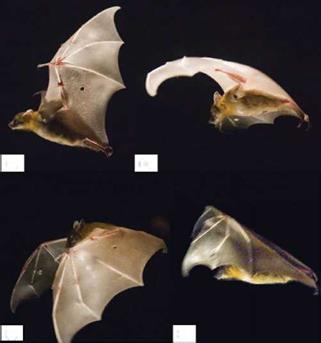
As discussed in Section 1.1, it is well known that flying animals typically have flexible wings to adapt to the flow environment. Birds have different layers of feathers, all of which are flexible and often connected to each other. Hence, they can adjust the wing planform for a particular flight mode. Furthermore, bats have more than two dozen independently controlled joints in the wing [400] and highly deforming bones [401] that enable them to fly at either positive or negative AoAs, to dynamically change wing camber, and to create complex 3D wing topology to achieve extraordinary flight performance. Bats have compliant thin-membrane surfaces, and their flight is characterized by highly unsteady and 3D wing motions (see Fig. 4.1).
As discussed in Chapter 1, birds and bats can also change their wingspan (flexing their wings) to decrease the wing area, increase the forward velocity, or reduce drag during an upstroke. In fast forward flight, birds and bats reduce their wing area slightly during the upstroke relative to the downstroke. At intermediate flight speeds, the flexion during the upstroke becomes more pronounced. However, bats and birds flex their wings in different manners. The wing surface area of a bird’s wing consists mostly of feathers, which can slide over each other as the wing is flexed and still maintain a smooth surface. Bat wings, in contrast, are mostly a thin membrane supported by the arm bones and the enormously elongated finger bones. Given the stretchiness of the wing membrane, bats can flex their wings a little, reducing the span by about 20 percent, but they cannot flex their wings too much or the wing membrane will go slack. Slack membranes are inefficient, because drag goes up and the trailing edges are prone to flutter, making them harder for fast flight [22].
While making bending or twisting movements, biological flyers have natural capabilities of adjusting the camber of their wings in accordance with what the flow environment dictates, such as a wind gust, object avoidance, and target tracking. Bats are known for being able to change the shape of the wing passively, depending on the free-stream conditions. As shown in Figure 4.1 bats can change their wing shapes during each flapping cycle. In human-made devices, sails and parachutes operate according to similar concepts. This passive control of the wing surface can prevent flow separation and enhance lift-to-drag ratio. Birds adjust their wings based on different strategies. For example, some species have coverts that act as self-activated
![]()
 (d)
(d)
Figure 4.1. A bat (Cynopterus brachyotis) in flight. (a) Beginning of downstroke, head forward, tail backward: the whole body is stretched and lined up in a straight line. (b) Middle of downstroke: the wing is highly cambered. (c) End of downstroke (also beginning of upstroke): the wing is still cambered. A large part of the wing is in front of the head and the wing is going to be withdrawn to its body. (d) Middle of upstroke: the wing is folded towards the body. FromTian et al. [231].
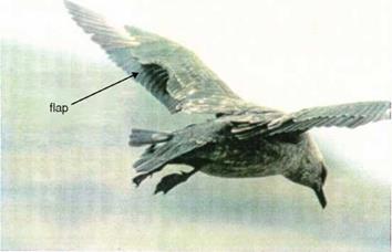
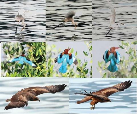
flaps to prevent flow separation. These features offer shape adaptation and help adjust the aerodynamic control surfaces; they can be especially helpful during landing and in an unsteady environment. In Figure 4.2 the coverts have popped up on a skua, and the flexible structure of the feathers is clearly shown. Figure 4.3 highlights three flyers in different flight modes: an egret fishing, a kingfisher trying to land, and a Black Kite during cruising.
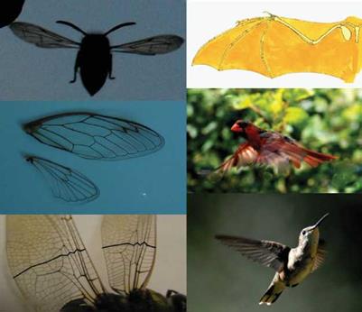
Insect wings deform to a great extent during flight, and their wing properties are generally anisotropic because of the membrane-batten structures; the spanwise bending stiffness is about 1 to 2 orders of magnitude larger than the chordwise bending stiffness in a majority of insect species. Experimental efforts reported a scaling relationship between wing flexural stiffness and wing length scale [402] [ 403]. In Combes and Daniel’s analysis each flexural stiffness is estimated based on a 1D beam model. The results showed that spanwise flexural stiffness scales with the third power of the wing chord, whereas the chordwise stiffness scales with the second power of the wing chord [402]. Figure 4.4 shows wings of cardinals, hummingbirds, bats, dragonflies, cicadas, and wasps, all exhibiting similar overall structural characteristics. They exhibit substantial variations in ARs and shapes, but share a common feature of a reinforced leading edge. A dragonfly wing has more local variations in its structural composition and is more corrugated than the wing of a cicada or a wasp. It was shown in the literature that wing corrugation increases both warping rigidity
|
Figure 4.2. The flexible covert feathers acting like self-activated flaps on the upper wing surface of a skua. Photo from Bechert et al. [416]. |
and flexibility [24]. The wing structure of a dragonfly helps prevent fatigue fracture [24].
Moreover, wing flexibility can allow for a passive pitching motion due to the inertial forces during the wing rotation as the stroke reverses [303]. There are three modes of passive pitching motion that are similar to those considered in the studies of rigid wing models (see also Fig. 3.9) [201] [245] [301]: (i) delayed pitching, (ii) synchronized pitching, and (iii) advanced pitching. The ratio of flapping frequency to the natural frequency of the wing is key to determining the modes of the passive pitching motion of the wing [404]. The thin nature of the insect wing skin structure makes it unsuitable for taking compressive loads, which may result in skin wrinkling and/or buckling. On the aerodynamics side, for example, wind-tunnel measurements show that corrugated fixed wings are aerodynamically insensitive to the Reynolds number variations, which is quite different from a typical low Reynolds number airfoil (see Section 3.5). For example, Figure 2.5 shows that a dragonfly wing is insensitive to the variation of the Reynolds number in its operating range, in contrast to the Eppler 374 airfoil, which displays a zigzag pattern at a certain Reynolds number range. Obviously, these features go beyond the fact that, as a flyer’s size is reduced, the wing becomes thinner and tends to become more flexible. As discussed in detail, the flexibility of the wing has a profound impact on its performance in lift, drag, and thrust. Fundamentally, a passively compliant structure can help adjust the structures so that the resulting aerodynamics can remain desirable [405]-[408]. Realizing that the dimensionless scaling of both fluid dynamics and structural dynamics (and their interactions) cannot be invariant, instead of trying to map out all physical mechanisms versus different Reynolds numbers and sizes, frequencies, and the like, one needs to focus on identifying favorable combinations of materials (elasticity, anisotropy, spatially varying properties, and so on) and on controlling the shape deformation of combined flapping and flexible structural dynamics, with the goal of identifying the most optimized combination of the kinematics, structural behavior, and possible control strategies (including hovering and wind gust effects).
|
Figure 4.3. Flexible wing patterns of three flyers in different flight modes, including an egret as a predator, a kingfisher trying to land, and a Black Kite during cruising. |
Overall, biological flyers have several outstanding features that may pose several design challenges in the design of MAVs. For example, (i) there is substantial anisotropy in the wing structural characteristics between the chordwise and spanwise directions; (ii) they employ shape control to accommodate spatial and temporal flow structures; (iii) they accommodate wind gust and accomplish station keeping with varying kinematics patterns; (iv) they use multiple unsteady aerodynamic mechanisms for lift and thrust enhancement; and (v) they combine sensing, control, and wing maneuvering to maintain not only lift but also flight stability. In principle, one might like to first understand these biological systems, abstract certain desirable features, and then apply them to MAV design. A challenge is that the scaling of fluid dynamics, structural dynamics, and flight dynamics between smaller natural flyers and practical flying hardware/lab experiments (larger dimension) is fundamentally difficult. Regardless, to develop a satisfactory flyer, one needs to meet the following objectives:
• Generate necessary lift, which scales with the vehicle/wing length scale as L3ef (under geometric similitude); however, often, a flyer needs to increase or reduce lift to maneuver toward/avoid an object, resulting in the need for substantially more complicated considerations
• Minimize power consumption
 Bat
Bat
Wasp
Cardinal
Cicada
Hummingbird
Dragonfly
Figure 4.4. Flexible and selectively stiffened wings of a cardinal, hummingbird, bat, dragonfly, cicada, and wasp.
As illustrated in Section 1.1, when wind gust adjustment, object avoidance, or station keeping become major factors, highly deformed wing shapes and coordinated wing – tail movement are often observed (see Fig. 1.12). Understanding of the aerodynamic, structural, and control implications of these modes is essential for the development of high-performance and robust MAVs capable of performing desirable missions. The flexibility of animal wings leads to complex fluid-structure interactions, whereas the kinematics of flapping and the spectacular maneuvers performed by natural flyers result in highly coupled non-linearities in fluid mechanics, aeroelasticity, flight dynamics, and control systems. Can large flexible deformations provide a better interaction with the aerodynamics than those limited to the linear regimes? If torsion stiffness along the wingspan can be tailored, how does that affect the wing kinematics for optimum thrust generation? How do these geometrically non-linear effects and the anisotropy of the structure affect the aerodynamics characteristics of the flapping wing?
Interaction between air and a thin structure is not only observed in animal locomotion. For example, the lift enhancement due to LEV formation that is discussed in the context of unsteady aerodynamic mechanisms in Chapter 3 is observed for autorotating plant seeds [409]. Freely falling papers [410] and their characteristic rotations that are typical for business cards or leafs [411] [412] are also well modeled with the principles described in Chapter 3. More recently, deformations of a leaf and the flow field around it have been measured at different wind speeds in a wind tunnel [413] (see also Fig. 4.5). The leafs reconfigure themselves by streamlining their structure such that the resulting drag grows slower than the classical U2
Figure 4.5. Six-inch (15-cm) MAV with flexible wing; from Ifju et al. [17].
 relations [414]. The vibration of the trees due to strong wind is one of the main reasons why trees are damaged, and uncovering these daily life physics helps us meet our environmental challenges.
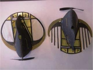
Nature’s design of flexible structures can be put into practice for MAVs. Adopting a flexible wing design (see Figs. 4.6 and 4.7) similar to bat wings can improve the performance of MAVs, especially at high AoAs by passive shape adaptation, which results in delayed stall [147] [ 406]. Figure 4.8, adapted from Waszak et al. [406], compares the lift curves versus AoAs for rigid and membrane wings. The three different flexible wing arrangements are depicted in Figure 4.7. The one-batten design has the most flexibility characterized by large membrane stretch. The two-batten design is, by comparison, stiffer and exhibits less membrane stretch under aerodynamic load. The six-batten wing is covered with an inextensible plastic membrane that further increases the stiffness of the wing and exhibits less membrane deformation and vibration. The nominally rigid wing is constructed with a two-batten frame covered with a rigid graphite sheet. Under modest AoA, both rigid and membrane wings demonstrate similar lift characteristics, with the stiffer wings having a slightly higher lift coefficient. However, a membrane wing stalls at a substantially higher AoA than a rigid wing. This aspect is a key element in enhancing the stability and agility of MAVs.
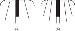 Figure 4.6. Three versions of the flexible wing were tested in the wind tunnel; from Waszak et al. [406]. (a) One-batten flexible wing; (b) two-batten flexible wing; and (c) six-batten flexible wing covered with an plastic inextensible membrane.
(c)
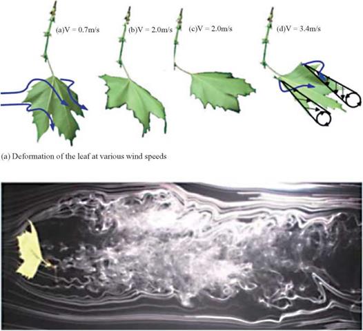 |
(b) Smoke-wire visualation of the flow behind a leaf at the AoA of 90°.
![Подпись: -•— Rigid (Graphite) Figure 4.8. Aerodynamic parameters vs. angle of attack for configurations with varying wing stiffness: (a) lift coefficient versus angle of attack; (b) lift-to-drag ratio versus the angle of attack. From Waszak et al. [406].](/img/3131/image366_2.gif) |
Figure 4.7. Aeroelastic study of a leaf in controlled laboratory setting. From Shao et al. [413].
|
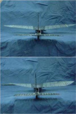
Figure 4.9. Representative MAVs with membrane wing developed by Peter Ifju and collaborators at the University of Florida. Left: the wing is framed along the entire peripherals. Right: the wing is flexible along the trailing edge while reinforced by battens. |
The membrane concept has been successfully incorporated in MAVs designed by Ifju et al. [17] and Stanford et al. [407]. However, traditional materials such as balsawood, foam, and monocoat, are not appropriate for implementing the flexible wing concept on these small vehicles. In their design illustrated in Figure 4.6 and Figure 4.9, unidirectional carbon fiber and cloth prepreg materials are used for the skeleton (leading-edge spar and chordwise battens). These are the same materials used for structures that require fully elastic behavior yet undergo large deflections. The fishing rod is a classic example of such a structure. For the membrane, extensible material is chosen to allow for deformations even under very small loads, such as for lightly loaded wings. Latex rubber sheet material has been used in this case. The stiffness of the whole structure can be controlled by the number of battens and the membrane material used.
As presented earlier, the experimental data for rigid and flexible wings (Fig. 4.8), with configurations similar to that shown in Figure 4.9, show that a membrane wing stalls at a substantially higher AoA than a rigid wing. Some aspects of low AR, low Reynolds number, and rigid wing aerodynamics have been presented by Torres and Mueller [162] as well as in Chapter 2. The lift-curve slope in Figure 4.8 is approximately 2.9 with the prop pinned. The lift-curve slopes of similar rigid wings reported by Torres and Mueller [162] at a comparable Reynolds number and aspect ratio (Re = 7 x 10⁴, AR = 2) are approximately 2.9 as well. However, these wings have stall angles between 12° and 15°. The stall angles of the flexible wings are between 30° and 45° and are similar to those of much lower aspect ratio rigid wings (AR = 0.5 to 1.0) [159]. However, low-aspect-ratio rigid wings exhibit noticeably lower lift-curve slopes, typically between 1.3 and 1.7 [159]. Hence, flexible wings can effectively maintain the desirable lift characteristics with better stall margins [406]. Figure 4.8 shows fixed, flexible-wing MAVs designed by Ifju and co-workers of the University of Florida [17]. The general specifications of the design are presented in Table 4.1. Stanford et al. [407] and Shyy et al. [408] reviewed the development of membrane-based fixed wing MAVs.
Figure 4.10. The flexible wing allows for wing warping to enhance vehicle agility [415].
 From an engineering point of view, flexibility can be used for purposes other than flight quality improvement. These objectives include shape manipulation and reconfiguration for both improved maneuvering and storage. Traditional control surfaces such as rudders, elevators, and ailerons have been used almost exclusively for flight control. By morphing or reshaping the wing using distributed actuation such as piezoelectric and shape memory material, preferred wing shapes can be developed for specific flight regimes. Such reconfiguration, however, would require substantial authority and power if the wings are nominally rigid. The flexible nature of the wing allows for such distributed actuation with orders of magnitude less authority. For example, the individual battens on the wing can be made from shape memory alloys, piezoelectric materials, or traditional actuators, such as servos, which can be used to manipulate the shape and properties of the wing.
Figure 4.10 illustrates a model with morphing technology. It employs a thread connecting the wingtips to a servo in the fuselage of the airplane. As the thread is tightened on one side of the aircraft, it acts like an aileron and causes the AoA of the wing to increase. The roll rate developed by such an actuation mechanism is considerably higher than that from a rudder. Additionally, it produces nearly pure roll with little yaw interaction. Detailed information on the related technical approaches has been presented by Garcia et al. [415].
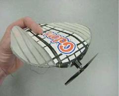
In some applications, it is desirable to store MAVs in small containers before releasing them. Flexible wing MAVs can be easily reconfigured for storage purposes. Figure 4.11 illustrates a 28 cm (11 inch) wingspan foldable wing MAV that can be
Figure 4.11. A foldable wing to enhance MAV portability and storage (Courtesy Peter Ifju).
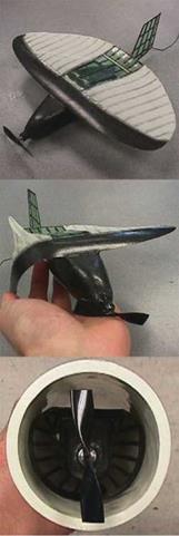 stored in a 7.6 cm (3 inch) diameter canister. The wing uses a curved shell structural element on the leading edge, which enables the wing to readily collapse downward for storage, yet maintain rigidity in the upward direction to react to the aerodynamic loads. The effect is similar to that of a common tape measure, where the curvature in the metallic tape is used to retain the shape after it has unspooled from the casing, yet it can be rolled back into the casing to accommodate the small-diameter spool. The curvature ensures that the positive (straight) shape is developed after it is unwound from the case and can actually be cantilevered for some distance. The curvature of the leading edge of the wing acts as the curvature in the tape measure.
This chapter highlighted the rigid flapping-wing aerodynamics at the low Reynolds number range between O(102) and O(104). Similar to a conventional delta wing,
|
Normalized pressure gradient |
|
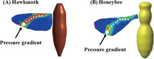
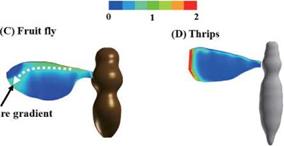
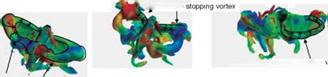
Figure 3.64. Spanwise pressure gradient contours on flapping wings around the middle of the downstroke: (A) a hawkmoth model (Re = 6.3 x 10³, k = 0.30); (B) a honeybee model (Re = 1.1 x 10³, k = 0.24); (C) a fruit fly model (Re = 1.3 x 10², k = 0.21), and (D) a thrips model (Re = 1.2 x 101, k = 0.25), respectively. |
a flapping wing can enhance lift because the vortex flow initiates at the leading edge of the wing, which rolls into a large vortex over the leeward side, containing a substantial axial velocity component. In both cases, vortex breakdown can occur, causing the destruction of the tight and coherent vortex. The LEV is a common feature associated with low Reynolds number flapping-wing aerodynamics; the flow structures are influenced by the swirl strength, the Reynolds number, and the rotational The effectiveness of LEVs in promoting lift is correlated with a flyer’s size. It seems that, at a fixed AoA, if the swirl is strengthened, then vortex breakdown occurs at lower Reynolds numbers. In contrast, a weaker swirling flow tends to break down at a higher Reynolds number. Hence, since the fruit fly, which operates at a lower Reynolds number range, exhibits a weaker LEV, it tends to better maintain the vortex structure than a hawkmoth and a honeybee, which create a stronger LEV. Furthermore TiVs associated with fixed finite wings are traditionally seen as phenomena that decrease lift and induce drag [297]. However, for flapping wings, the wing and vortex interactions, and consequently the aerodynamic outcome, can be far more complex. For a low-aspect-ratio hovering wing, with delayed rotation, TiVs can increase lift both by creating a low-pressure region near the wingtip and by anchoring the LEV to delay or even prevent it from shedding. Furthermore, for certain flapping kinematics such as synchronized rotation with modest AoA, the LEV remains attached along the spanwise direction and the tip effects are not prominent; in such situations, the aerodynamics is little affected by the AR of a wing. Appropriate combinations of advanced rotation and dynamic stall associated with large AoAs can produce more favorable lift. The combined effects of TiVs, LEV, and jet can be manipulated by the choice of kinematics to make a 3D wing aerodynamically better or worse than an infinitely long wing. Furthermore, the delayed stall of the LEV and interaction of TiVs and LEVs are significantly affected by the free – stream.
However, wing-wake interactions and TiVs can lead to a decrease in the aerodynamic performance when the wing orientation and the surrounding vortical flow structure are not well coordinated. Hence, the effectiveness of the unsteady flow mechanisms is strongly linked to the flapping wing kinematics, Reynolds number, and the free-stream environment.
This chapter also assessed the roles of Re, St, k, as well as kinematics at the Reynolds number of O(104), for both flat plate and SD7003 airfoil in forward flight with a shallow stall (pitch/plunge) and a deep stall motion (plunge). Massive leading – edge separation is observed at the sharp leading edge of the flat plate; its geometric effect is seen to dominate over other viscosity effects and the Re dependence is limited. For the blunter SD7003 airfoil, the flow is mostly attached for the shallow stall motion at Re = 6 x 10⁴, whereas it experiences massive separation for the deep stall motion. The deep stall kinematics produces a more aggressive time history of effective AoA with a higher maximum. The flow is characterized by a stronger leading-edge separation with earlier generation of an LEV and formation of a secondary vortex near the surface of the flat plate. The maximum lift coefficients of the flat plate are substantially different from those for the SD7003 airfoil. Furthermore, there is a noticeable phase lag in the deep stall SD7003 airfoil and flat plate in the time history of the lift coefficient. The difference in curvature of the leading-edge shape causes the lag in the generation and evolution of the LEV. Overall, for the shallow stall motion, the force acting on the SD7003 airfoil has smaller lift and drag compared to the force on the flat plate due to the formation of an LEV in the flat plate case. In contrast, the shape effects become less significant for the deep stall motion with higher maximum effective AoA: the flow separates over the SD7003 airfoil during the latter half of the downstroke, and the resulting force is similar to that of the flat plate.
The studies based on the kinematics and geometries of biological flyers offer direct evidence of unsteady aerodynamic mechanisms. Compared to flow structures generated by simple flapping motion, those around insect flapping wings have unique features, such as ring-like vortex generation per stroke with a strong downward jet.
We also highlighted selected linearized aerodynamic models used for control applications or design optimizations because their computational cost is significantly smaller than that of Navier-Stokes equation solutions; however, their applicability is not comprehensively understood in the flapping wing regime. Whereas quasi-steady models tend to over-predict the lift generation and may not able to capture wing – wake interactions with varied Reynolds numbers, they can still provide reasonable time-averaged lift estimations.
The chapter also presented several studies focusing on biological flyers, aimed at offering case studies in nature, as well as snapshots of interesting flow characteristics discussed in “canonical” investigations based on simplified problem definitions.
The topics discussed and highlighted in this chapter are essential to understand flapping wing aerodynamics with rigid wings. In Chapter 4 we discuss the effects of wing flexibility that increases the degree of freedom and showcase the challenges and intriguing features of multidisciplinary physics.
As discussed previously, the lift enhancement due to the delayed stall of the LEV is important in flapping wing flight [199] [245]. The formation of the LEV depends on the wing kinematics, the details of wing geometry, and the Reynolds number [397]. To examine the Re effect on LEV structures and spanwise flow for insect-like wing body configurations with appropriate kinematic motions, Shyy and Liu [397] and Liu and Aono [225] investigated the flapping wing fluid physics associated with the hawkmoth (Re = 6.3 x 10³, k = 0.30), honeybee (Re = 1.1 x 10³, k = 0.24), fruit fly (Re = 1.3 x 10², k = 0.21), and thrips (Re = 1.2 x 101, k = 0.25) in hover. Different representative kinematic parameters (flapping amplitude, flapping frequency, and type of prescribed actuation) and
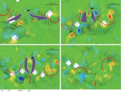 Figure 3.62. Hovering Japanese White-eye wake flow fields on a frontal plane. Color contours represent the vorticity distribution of the flow fields. (a-c) Near-wake flow fields pertaining to kinematic phases of the ventral clap; purple patches mark the position of the two wings, and purple dotted lines indicate an outline of the bird. (d) The far-wake flow field beneath a hovering Japanese White-eye after phase 3; thick red arrows depict the trends of the flow motion. (a-d) Thick red arrows show the trends of flow motions. (e) Schematic sketches summarizing the wake flow structures for the three kinematic phases. Black arrows indicate fluid jets; orange and blue spiral arrows represent, respectively, the LEV and TEV. Purple arrows signify the downward jet generated by the downstroking wings executing the ventral clap. From Chang et al. [391].
dimensionless numbers (Reynolds number, reduced frequency) are considered for each insect model [225]. The Reynolds number and reduced frequency are calculated based on mean chord and tip velocity. The morphological and kinematical model of a hawkmoth was already shown in Figure 3.56 and Figure 3.57. For other insect models, similar information and computational models can be obtained in Liu and Aono [225].
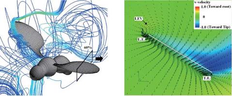
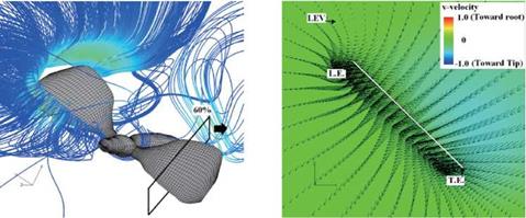
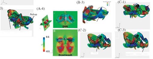
Figure 3.63 shows the velocity vector field on an end-view plane at 60 percent semi-span for these four insects. The LEV structure and the spanwise flow in the hawkmoth and the fruit fly cases (see Fig. 3.63A and C) are in good qualitative agreement with the corresponding experimental results reported in Birch et al. [283]. For the thrips (Re = 1.2 x 101, к = 0.25), the LEV forms upstream of the leading edge, and spanwise flow is weakest among all cases. For the fruit fly (Re = 1.3 x 10², к = 0.21), the LEV structure is smaller than that of the hawkmoth
 |
and the honeybee. The fruit fly LEV is tube-like and ordered, and spanwise flow is observed around the upper region of the trailing edge. The hawkmoth (Re =
6.3 x 10³, к = 0.30) and honeybee (Re = 1.1 x 10³, к = 0.24) cases yield much more pronounced spanwise flow inside the LEV and upper surface of the wing, which together with the LEV forms a helical flow structure near the leading edge (see Fig. 3.63A-1 and B-1). Figure 3.64 shows the spanwise pressure gradient contours on the wing of four typical insects at the middle of the downstroke. Compared to the hawkmoth and the honeybee, even though the wing kinematics and the wing-body geometries are different, fruit flies, at a Re of 1.0 x 10²~2.5 x 10², cannot create as steep pressure gradients at the vortex core; nevertheless, they seem to be able to maintain a stable LEV during most of the down – and upstroke. Although the LEVs on both the wings of the hawkmoth and honeybee experience a breakdown near the middle of the downstroke, the LEV on the fruit fly’s wing remains attached during
|
(C-1) Streamlines (C-2) Spanwise flow |
|
(C) Fruitfly model (Re= 1.3×10², k=0.21)
(D-1) Streamlines (D-2) Spanwise flow (D) Thrips model (Re= 1.2×101, k=0.25) Figure 3.63 (continued) |
the entire stroke, eventually breaking down during the subsequent supination or pronation [387].
In reality the thrips wings are extremely small – of the order of 1 mm – and are composed of a comblike planform with solidity ratios of 0.2 and less [398]. Consequently, the Reynolds numbers are so low that the viscous effects dominate and the unsteady viscous flow around their wings can be approximated as Stokes flow. Using slender-body theories the flow physics around an array of oscillating bodies was studied by Weihs and Barta [398] and Barta [399]. They showed that the comblike wings of thrips are able to produce forces similar to those of solid wings, while being able to save weight.
According to their kinematic characteristics, the modes of bird-hovering flight are typically classified as symmetric, notably employed by hummingbirds, and asymmetric, which is often observed in other birds, such as the Japanese White-Eye (Zosterops japonicus) and Gouldian Finch (Erythrura gouldiae), both of which belong to the order Passeriforme. For a hovering passerine, only the downstroke produces the lift force necessary to support the bird’s weight; the upstroke is aerodynamically inactive and produces no lift [4] [389] [390]. Hence, even without producing lift forces continuously throughout the entire cycle of wing beating, a passerine is able to hover.
Chang et al. [391] presented experimental measurements to support the notion that a hovering passerine (Japanese White-Eye, Zosterops japonicus) can employ an unconventional mechanism of “ventral clap” to produce lift for weight support. They claimed that this ventral clap can first abate and then augment lift production during the downstroke. The net effect of the ventral clap on lift production is positive because the extent of lift augmentation is greater than the extent of lift abatement, as shown in Figure 3.62, where the PIV data illustrate the flow structures associated with the various phase of the flapping motion. As discussed in this section and by Trizila et al. [301], LEV and TEV flows as well as the downward jet flow are observable, contributing to the complicated balancing and net generation of aerodynamic forces.
In Chang et al.’s study [391], two methods based on wake topology were applied to evaluate the locomotive forces. The first is primarily associated with the Kutta – Joukowski lift theorem [392]-[394]. For a bird executing quasi-steady level flight, the total lift acting on its wings must be equal to its weight. The second method to evaluate the locomotive force is based on a vortex-ring model that obtains a time – averaged force from a calculation of the momentum change (i. e. impulse), divided by the generation period of a vortex ring shed by a flapping or beating appendage of a locomoting animal [342] [395] [396]. Although these methods are simple and convenient, as discussed in Section 3.6, such approaches encounter difficulties in offering an accurate account and they are not based on first principles.
Figures 3.56 and 3.57 show the morphological and wing kinematics models of a realistic hawkmoth model. Computations were performed by Liu and co-workers using “a biology-inspired dynamic flight simulator” [387] [388].
3.7.1.1 Vortical Structures and Lift Generation
Iso-vorticity-magnitude surfaces around a hovering hawkmoth at selected instants during a flapping cycle are shown in Figure 3.58. The contour color on the iso- vorticity-magnitude surfaces in Figure 3.58 indicates the magnitude of the normalized helicity density. The corresponding time histories of the vertical force on the wings and body are plotted in Figure 3.60.
flow structures during downstroke. In the first half of the downstroke as indicated at point (a) in Figure 3.57, a horseshoe-shaped vortex is generated by the initial wing motion of the downstroke (see Fig. 3.58A-1. Poelma et al. [270] showed a similar 3D flow structure around an impulsively started dynamically scaled flapping wing using PIV (see Fig. 3.59). The horseshoe-shaped vortex is composed of three vortices – an LEV, a TEV, and a TiV – and it grows in size as the translational and angular velocity of the wing increases. These vortices produce a low-pressure region in their core and on the upper surfaces of the wing (Figure 3.61, section 1) when they are attached. Lift forces show a peak at the corresponding time instant (point (b)
![]()
 |

 Doughnut-shaped vortex ring
Figure 3.58. Visualization of flow fields around a hovering hawkmoth. Iso-vorticity-magnitude surfaces around a hovering hawkmoth during (a) the downstroke, (b) the supination, and (c) the upstroke, respectively. The color of iso-vorticity-magnitude surfaces indicates the normalized helicity density, which is defined as the projection of a fluid’s spin vector in the direction of its momentum vector, being positive (red) if these two vectors point in the same direction and negative (blue) if they point in the opposite direction.
Figure 3.59. 3D horseshoe-shaped vortex indicated with an iso-Q – surface around an impulsively started wing. The contours on the wing represent the vorticity with its direction indicated by the arrows. From Poelma et al. [270].
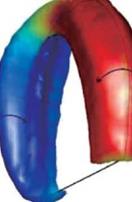 in Fig. 3.57). As expected, coherent LEVs, TEVs, and TiVs together enhance the lift generation in hovering flight of the hawkmoth. During the mid-downstroke (see point (c) in Fig. 3.57), the TEVs shed mostly from the wings while on the body they stay attached. Moreover, the shed TEVs stay connected to the TiVs (Fig. 3.58A-2). Overall, the LEVs produce the largest and strongest area of low pressure on the wing surface (Fig. 3.61, section 2). Shortly afterward, the LEVs begin to break down at a location approximately 70-80 percent the span of the wing length. At the same time, the LEV, the TiV, and the shed TEV together form a doughnut-shaped vortex ring around each wing (Fig. 3.58A-3). Similar vortex ring structures have been observed around a hovering hummingbird [261] [266], a bat in slow forward flight [268], and a free-flying bumble bee [259]. During the second half of the downstroke (see point (d) in Fig. 3.57), the TiVs enlarge and weaken. As the wings approach the end of the downstroke, both LEVs and TiVs begin to detach from the wings. During most of the downstroke, the doughnut-shaped vortex ring pair has an intense, downward jet flow through the “doughnut” hole, which forms the downstroke downwash (see Fig. 3.58A-4).
While approaching supination (see point (e) in Fig. 3.57), the flapping wing slows down, and the attached vortices are shed from the wings. At this time instant, a pair of downstroke stopping vortices is observed wrapping around the two wings (Fig. 3.58B-1). When the flapping wings begin to pitch quickly about the spanwise axis,
![]()
![]()
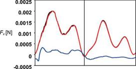
![]() Figure 3.60. Time courses of vertical force of a hovering hawkmoth model over a flapping cycle. t/T = 0-0.5 corresponds to the down – stroke. Black, red, and blue lines represent the aerodynamic forces acting on the right wing, left wing, and body, respectively. The weight of a hawkmoth is around 15.7 x 10³ [N] [384].
Figure 3.60. Time courses of vertical force of a hovering hawkmoth model over a flapping cycle. t/T = 0-0.5 corresponds to the down – stroke. Black, red, and blue lines represent the aerodynamic forces acting on the right wing, left wing, and body, respectively. The weight of a hawkmoth is around 15.7 x 10³ [N] [384].
|
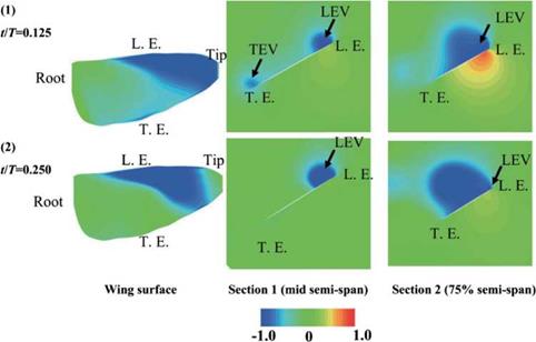
Figure 3.61. Pressure distributions at selected time instants corresponding to Figure 3.57 (b) and (c) during the downstroke. Left: Upper wing surface. Middle: Mid semi-span crosssection. Right: 75% semi-span cross-section from the wing root. Note that L. E. and T. E. indicate leading edge and trailing edge, respectively. Note that the pressure coefficients in the LEV are negative in all sub-figures. |
a pair of upstroke starting vortices is detected around the wingtip and the trailing edge (Fig. 3.58B-2).
flow structures during upstroke. After supination (point (f) in Fig. 3.57), TEVs and TiVs associated with the beginning of the upstroke are generated when the flapping wings rapidly accelerate. The downstroke wakes of the circular vortex rings are subsequently captured (Fig. 3.58B-3), but only a minor impact on lift is seen (Fig. 3.60). As discussed in Section 3.3, the role of the unsteady flow structures on lift enhancement needs to be examined in specific context. As the upstroke starts, (point (g) in Fig. 3.57), the TEVs and TiVs are shed from the two wings (Fig. 3.58C-1). Together with the TEVs, the LEVs and TiVs form a horseshoe-shaped vortex pair wrapping each wing (Fig. 3.58C-2). Similar to what is seen during the downstroke, the horseshoe-shaped vortex grows and evolves into a doughnut-shaped vortex ring for each wing. It should be pointed out that, due to asymmetric variation of the AoA between the upstroke and downstroke, the LEVs generated in the upstrokes are smaller than those in the downstroke. Late in the upstroke (point (h) in Fig. 3.57), the doughnut-shaped vortex rings elongate and deform while maintaining their ring-like shape (Fig. 3.58C-3).
As for the aerodynamic force generation, two peaks in the lift force are predicted during each stroke for a hovering hawkmoth (see Fig. 3.60). Considering the correlation between the aerodynamic forces and the key unsteady flow features associated with flapping wings discussed in Section 3.3, the delayed stall of the LEV and contributions from the TEV and TiV are responsible for the first lift peak. The
second peak is likely to be associated with a contribution from the rapid increase in vorticity [289] as the wing experiences a fast pitching motion.
As discussed in the previous section, the helicopter blade model has been used to help explain the flapping wing aerodynamics; however, spanwise axial flows are generally considered to have a minor influence on the helicopter aerodynamics [289] [375]. In particular, helicopter blades operate at a substantially higher Reynolds number and lower AoA than flapping wings. The much larger AR of a blade also makes the LEV harder to anchor. These are key differences between helicopter blades and typical biological wings.
Usherwood and Ellington [320] investigated the aerodynamic performance associated with “propeller-like” rotation of the hawkmoth wing model (Re = 0(103)). They reported that revolving models produced high lift and drag forces because of the presence of the LEV. Knowles et al. [376] performed computational studies involving with translating 2D and rotating 3D flat plate models at Re = 5.0 x 10². Their results showed, that for 2D flows, the LEV is unstable, but the rotating 3D flat plate model at high AoA produces a conical LEV, as observed in the results presented earlier and by others [320] [377]. Moreover, they noted that if the Reynolds number increases above a critical value, a Kelvin-Helmholtz instability [378] occurs in the LEV sheet, resulting in the sheet breaking down on outboard sections of the wing.
Lentink and Dickinson [379] revisited existing hypotheses regarding stabilizing the LEV. Using a fruit fly wing model, they systematically investigated the effects of propeller-like motion on aerodynamic performance and LEV stability at Re = 1.1 x 10²-1.4 x 10⁴ based on theoretical and experimental approaches. They stated that the LEV is stabilized by the “quasi-steady” centripetal and Coriolis accelerations that are present at low Rossby numbers (i. e., a half of the AR) and result from the propeller-like sweep of the wing. In addition, they suggested that the force augmentation through a stably attached LEV could represent a convergent solution for the generation of high fluid forces over a range of Reynolds numbers.
Jones and Babinsky [380] experimentally examined unsteady lift generation on rotating wings with AoA of 5° and 15° at a Reynolds number of 6.0 x 10⁴. A transient high list peak, approximately 1.5 times the quasi-steady value, occurred in the first chord length of travel, and it was caused by the formation of a strong LEV. They showed that wing kinematics has only a small effect on the aerodynamic force produced by the waving wing. In the early stages of the wing stroke, the velocity
![Подпись: Figure 3.56. A morphological model of a hawk- moth, Agrius convolvuli, with a computational model superimposed on the right half. The hawk- moth has a body length of 5.0 cm, a wing length of 5.05 cm (mean wing chord length cm = 1.83 cm), and an aspect ratio of 5.52. The image is from Aono, Shyy, and Liu [384].](/img/3131/image333_3.gif) |
 profiles with low accelerations affect the timing and the magnitude of the lift peak, but at higher accelerations, the velocity profile is insignificant.
From the viewpoint of unsteady aerodynamics, the LEV as a lift-enhancement mechanism at a higher Re range (0(105-106)) may be questionable because a dynamic stall vortex on an oscillating airfoil is often found to break away and to convect elsewhere as soon as the airfoil translates [277].
3.6 Modeling of Biological Flyers in a Rigid-Wing Framework
There are a number of computational studies based on realistic wing configurations of natural flyers, such as a hornet [381], bumblebee [382] [383], hawkmoth [200] [247] [384], honeybee [225], drone fly [385], hover fly [386], fruit fly [387], and thrips [225]. In following, we present selected examples to highlight some of the features discussed in previous sections, as well as to gain insight into how flow structures are associated with the specific characteristics of wing motion.
The aerodynamic theories described in the previous sections dealt with the linearized aerodynamic theories by assuming thin flat plates or by taking the quasi-steady
|
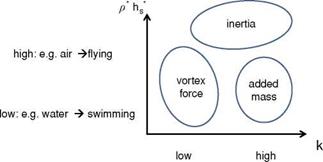
Figure 3.55. Schematic of the dominant mechanisms for force generation that is responsible for the wing deformation (see also Table 3.2) of a flexible flapping wing. Inertia force is the force acting on the wing due to the wing acceleration relative to the imposed motion at the wing root. |
assumption in inviscid flows. Exact solutions for the unsteady viscous flows described by the Navier-Stokes (see Eq. (3-18)), are unknown due to their non-linearity. Recently, numerical computations (e. g., [200] [296] [369]) and detailed experimental measurements (e. g., [199] [201] [323]) have revealed intriguing unsteady flow physics related to the flapping wing aerodynamics (see, e. g., Section 3). However, some key questions, such as the relation between the aerodynamic performance of flapping wings and the non-dimensional parameters introduced in Section 3.2, are still challenging.
Based on a control volume analysis of incompressible viscous fluid around a moving body [370] [371], Kang et al. [351] normalized the resulting hydrodynamic impulse term, which relates the vortices in the flow field to the force acting on the moving body, and the acceleration-reaction term, as shown in Eq. (3-35),
Cf = Cf, impulse + C^ ^ St O(1) + |o(1)j + StkO(1) (3-35)
as a first-order approximation. Note that the first term is independent of the motion frequency and the second term is proportional to 2n f. The force due to the hydrodynamic impulse scales with St. However, if the viscous time scale, c2mp/p-, is much greater than the motion time scale, 1/(2n f), such that Rek > 1, then the first term in Eq. (3-35) becomes negligible. Moreover, when the plunge amplitude ha/cm ~ St/k is small, the second term in Eq. (3-35) will make only a small contribution to the total force felt on the wing. In general, however, complex fluid dynamic mechanisms, such as the wing-wake interaction, or the wake – wake interactions would additionally affect the vorticity distribution in the flow field.
The last term of Eq. (3-35) is the acceleration-reaction term indicating the force due to the acceleration of the wing. When a body accelerates in a fluid, the fluid kinetic energy changes. The rate of work done by pressure moving the body yields the acceleration-reaction force. In an inviscid fluid this force is proportional to the acceleration (see, e. g., [372]). The constant of proportionality has the dimension of mass; hence, the name “added mass.” The added mass term is usually some fraction of the fluid mass displaced by the body. Determination of the added mass, which is a tensor because it relates the acceleration vector to the force vector, is not easy in general because the local acceleration of the fluid is not necessarily the same as the acceleration of the body [45]. However, for an accelerating thin flat plate with a chord length cm normal to itself, the force acting normal to the flat plate can be obtained as
PfFa = dt (pf 4 ’ (3-36)
where vi is the vertical velocity component: the added mass of a vertically accelerating thin flat plate is equal to the displaced fluid cylinder with radius cm/2. The added mass due to angular rotations can be obtained similarly, which results in the non-circulatory term as in Theodorsen, Eq. (3-21), or its quasi-steady approximation for the pure plunge motion, Eq. (3-22). Note also that the combination of non-dimensional numbers appearing in the previous formulas and in Eq. (3-35) is consistent.
This non-dimensionalization process reveals that the fluid dynamic force is proportional to St; hence, with increasing St, the force acting on the wing is expected to increase. Furthermore, if the motion is highly unsteady (i. e., к is high), the force due to the motion of the body, appearing as the acceleration-reaction component, dominates over the forces due to vorticity in the flow field.
A parametrization of special interest for the flapping wing community is the dependence of the force on the flapping motion frequency, m. The current scaling shows that for forward flight with Uref = UTO the acceleration-reaction force has the highest order of frequency as ~ (2n f )2. The resulting dimensional force is then proportional to the square of the motion frequency. Similarly, for hovering motions the current scaling shows that the non-dimensional force is independent of the motion frequency since the Strouhal number is a constant and the reduced frequency is only a function of flapping (plunging) amplitude. However, since Uref ~ (2n f )2 the resulting dimensional force is also proportional to the square of the motion frequency. Similar observations were reported by Gogulapati and Friedmann [367].
At a high Reynolds number, high reduced frequency regime, Visbal, Gordnier, and Galbraith [373] considered a high-frequency small amplitude plunging motion at Re = O(104) over a 3D SD7003 wing (a0 = 4 deg, к = 3.93, St = 0.06, Re = 1 x 10⁴ and 4 x 10⁴). They used the implicit LES approach to solve for the flow structures, including the laminar-to-turbulence transition and the forces on the wing. The flow field exhibits formation of dynamic stall features such as LEVs, breakdown due to spanwise instabilities, and transitional features; however the forces on the wing could still be well predicted by the Theodorsen [374] formula for lift. The time history of lift was “independent of Reynolds number and of the 3D transitional aspects of the flow field” [373]. Visbal and co-workers explained that the lift is dominated by the acceleration of the airfoil, which is proportional to the square of the motion frequency. This observation is also consistent with the fact that the scaling of the hydrodynamic impulse term is small compared to the acceleration-reaction term in Eq. (3-35) for the given non-dimensional parameters.
In contrast, at lower Reynolds numbers, Trizila et al. [301] showed at Re = 100 and к in the range of 0.25-0.5 that the formation and interaction of leading – edge and trailing-edge vortices with the airfoil and previous shed wake substantially affect the lift and power generation for hover and forward flight. Furthermore, three – dimensionality effects play a significant role. For instance, for a delayed rotation kinematics (к = 0.5, low angle of attack, Re = 100), the tip vortex generated at the tip of the AR = 4 flat plate would interact with the LEV, thereby enhancing lift compared to its two-dimensional counterpart; this is in contrast to the classical steady-state thin wing theory [301] [296] that predicts the formation of TiVs as a lift-reducing flow feature. This complex interplay between the kinematics, the wing-wake and wake – wake interactions, and the fluid dynamic forces on the wing at the given range of nondimensional parameters is also consistent with the scaling analysis described in this section as summarized in Table 3.2. The scaling shows that, for low reduced frequency motions or low Reynolds number flows, the hydrodynamic impulse term, which indicates the interaction between the vortices and the wing becomes important. In contrast, when the reduced frequency increases, the acceleration-reaction term dominates over the hydrodynamic impulse term. Both components are proportional to the Strouhal number. An interesting consequence that needs to be investigated
|
Table 3.2. Summary of the force scaling
|
more is that in the hovering flight condition where both the Strouhal number and reduced frequencies are independent of motion frequency, the normalized force will be independent of frequency for high Reynolds number flows.
The simplified models – such as Theodorsen’s formula for lift, Eq. (3-21) for forward flight, the revised quasi-steady model proposed by Sane and Dickinson [292], or Eq. (3-33) for hover – are very powerful for obtaining a quick estimate of lift generation or for design and optimization purposes, but they do not guarantee the accuracy of the solution. A solution from a Navier-Stokes equation solver would be more accurate, but it would take hours or even days to obtain one single 3D simulation. It is hence of great importance to assess when or why the simplified models give reasonably accurate results.
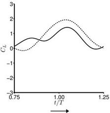
(a) Pitching and plunging (0.68, 0.89, 0.77) (b) Purely plunging (0.78, 0.79, 0.73)
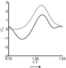
For the shallow stall and deep stall kinematics discussed in Section 3.5, the lift prediction by the Theodorsen formula Eq. (3-21) is plotted against the lift obtained by numerical computations for a 2D SD7003 airfoil and flat plate in Figure 3.50. For the shallow stall case, Theodorsen’s result matches the computations reasonably during the downstroke. The agreement improves in the second part of the upstroke. Although Eq. (3-21) is derived for a thin flat plate, the lift prediction is closer to that of SD7003 airfoil. This difference stems from the formation of LEV for the case of a flat plate as shown in Figure 3.33 during the downstroke. As the LEV convects downstream, the lower pressure region in the vortex core enhances the lift. Subsequently the LEV detaches and the flat plate loses the leading-edge suction. At t/T = 0.5 the discrepancy is the largest where the flow over the SD7003 experiences an open separation [323]. Since Theodorsen’s solution assumes a planar wake and Kutta condition at the trailing edge, the wake structure at t/T = 0.5 violates this condition, causing the discrepancy in the lift coefficient. Overall, Theodorsen’s solution approximates the lift coefficient from the numerical computation better when the wake is planar. In the deep stall, as discussed in Section 3.5 flow over both the SD7003 and flat plate separates early in the downstroke, leading to LEV formation. The resulting flow structures and the time history of lift are similar. Again, Theodorsen’s prediction gives a reasonable estimation, but is less accurate when an LEV is formed.
For the hovering flat plates, the quasi-steady lift predicted by Eq. (3-34) is compared to the numerically computed lift of hovering flat plates at Re = 100 for the cases highlighted in Section 3.4. Although the case setup is different (e. g., Dickinson et al. [201] used a revolving 3D wing, whereas Trizila et al. [301] used plunging flat plates), such a comparison highlights the usefulness and the limitations of applying quasi-steady models for design or control purposes. For these cases Eq. (3-34) captures the general trends well, but over-predicts the lift peak during the second part of the stroke, which is reflected in the time-averaged lift coefficients: the quasisteady values are greater than the computed values. Most notable differences are
found during the first part of the stroke where the returning flat plate interacts with the wakes shed in the previous stroke, as explained in Section 3.6.2. For the delayed rotation and both the synchronized rotation cases (Fig. 3.51a, c, d), the first lift peak that is due to wake capture is not captured at all by Eq. (3-34). In fact because the airfoil pitches down while accelerating forward, the rotational component, Fr, dominates and yields negative lift. For the advanced rotation case shown in Figure 3.51b, because the interaction with the downward wake [359] is not included in the quasi-steady model Eq. (3-34), the negative portion of the lift between t/T = 0.75 and 1.00 is not captured. The biggest difference in the predicted and computed time-averaged lift coefficient is found for the cases with these kinematics. The global trend is illustrated in Figure 3.52 where the time-averaged lift coefficients for all cases considered by Trizila et al. [301] are plotted with the x-coordinate being the quasi-steady model prediction given in Eq. (3-34) and the у-coordinate the Navier – Stokes computation from Trizila et al. [301]. It is clear that Eq. (3-34) over-predicts the mean lift, and for some cases the error can be huge (e. g., the case shown in Fig. 3.51b).
Gogulapati and Friedmann [367] extended Ansari’s unsteady aerodynamic model to forward flight and flexible wings and also incorporated a vorticity decay model to include the effects of viscosity. They compared their results to the numerical results shown in Section 3.4.1 and showed that the correlation indeed improves when the viscosity effects are included. They also investigated the role of LEV shedding. For the case where the 3D flow field is similar to the 2D flow field (Section 3.4), the vortical activity from the leading edge is small, as shown in Figure 3.27. For this case, Gogulapati and Friedmann’s model showed that the best correlation to the Navier – Stokes computations is obtained when an attached flow is assumed: the aerodynamic model is adjusted not to shed any vorticity from the leading edge. In contrast, for the delayed rotation with high AoA and low plunging amplitude case (Section 3.4.1.1), results with LEV shedding agree the best with the Navier-Stokes computations (see Fig. 3.53). For combined pitch and plunging motions in hover it was shown that the forces predicted by the approximate model match Navier-Stokes solutions reasonably well for a Zimmerman wing with the flapping amplitudes of 10° to 15° and the pitching amplitude of 5° and 10°. The motion frequency was fixed at 10 Hz, resulting in the reduced frequency of 1 to 1.5 based on the mean wingtip speed and Re of 0(103). The differences between this approximate model and the Navier-Stokes model were attributed to 3D effects at play, such as TiV generation, LEV-TiV interaction [296], or spanwise flow. Also for flapping Zimmerman wings in forward flight, the flapping amplitude was kept at 35° and the frequency at 10 Hz. By varying the advance ratio and hence the incoming free-stream velocity, they correlated the agreement between their result and the Navier-Stokes solutions to the advance ratio, which is inversely proportional to the reduced frequency. The agreement was more favorable for the higher reduced frequencies (see Fig. 3.54). A plausible reason for this effect is that, as shown in Section 3.6.4 for high reduced frequency and high Reynolds number flows, the added mass force dominates, which is related to the acceleration of the wing. As the reduced frequency decreases, the influence of the vortices in the flow field increases, which is harder to capture by potential theory-based approximate models.
-2.5 -2 -1.5 -1 -0.5 0 0.5 1 1.5 2 2.5 x
 |
(b) advanced rotation, low AOA (1.00/0.15)
 -2.5 -2 -1.5 -1 -0.5 0 0.5 1 1.5 2 2.5 x
(c) synchronized rotation, high AOA (0.85/0.65)
low AOA (0.54/0.14)
Figure 3.51. Lift coefficient during the forward stroke. —, Navier-Stokes equations (Re = 100); —, quasi-steady model as shown in Eq. (3-34). The time-averaged lift coefficients from the quasi-steady model and the computation are indicated in the parentheses.
Figure 3.52. Time-averaged lift coefficients predicted by the quasi-steady model given in Eq. (3-34) on the x-axis and the Navier – Stokes computations on the у-axis for hovering flat plates at Re = 100 [301].
![Подпись: Figure 3.53. Time history of forces from the approximated aerodynamics model [367] and the Navier-Stokes computation [301] for a hovering flat plate at Re = 100 (delayed rotation, high AoA). When the approximate aerodynamic model assumed separated flow, including viscous effects, the agreement improved. From Gogulapati and Friedmann [367].](/img/3131/image329_3.gif) |
Recently, Ol and Granlund [368] considered several flapping rigid-wing experiments in water: (i) a flat plate free to pivot around its leading edge under a periodic translational motion, (ii) linear pitch-ramp motion with varying pivot points, and (iii) a combined pitch-plunge. They conjectured that the aerodynamic force responses are not quasi-steady; that is, the lift is proportional to an effective angle of attack with the proportionality constant being some coefficient (e. g., 2n), but it can be modeled by including the second and the first derivatives of the effective angle of attack. Despite the inherent limitations of linearized aerodynamic models as discussed in this section, research in this area has been popular recently because of these models’ applicability to control applications or design optimizations. As is shown in Section 3.6.2, the quasi-steady model can be significantly improved if one can estimate the
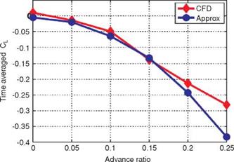
|
Figure 3.54. Time-averaged lift coefficients from the approximated aerodynamics model (blue circle) and the Navier-Stokes computations (red diamond) for a rigid Zimmerman wing in forward flight at Re = 4.6 x 10³, flap amplitude of 35°, and frequency of 10 Hz. The advance ratio is inversely proportional to the Strouhal number and also to the reduced frequency for fixed flap amplitude. From Gogulapati and Friedmann [367]. |
effective angle of attack, instead of the nominal value. For low Reynolds number, flapping wing aerodynamics, the viscous effect is significant, and the interaction between the wing and the surrounding large-scale vertical flows created by the wing motion in the previous and present strokes can noticeably affect the instantaneous actual angle of attack. Thus, in addition to the historical effects of the fluid physics, careful consideration of the quasi-steady framework is required before adopting it as a predictive tool.
Following the helicopter theory, a simplified analysis for flapping flight can be established based on the actuator disk model. An actuator is an idealized surface that continuously pushes air and imparts momentum to downstream by maintaining a pressure difference across itself (i. e., the lift is equal to the change in fluid momentum). Assuming that insect wings beat at high enough frequencies so that their stroke planes approximate an actuator disk, the wake downstream of a flapping wing can be modeled as a jet with a uniform velocity distribution [65] [338]. Although the momentum theory accounts for both axial and rotational changes in the velocities at the disk, it neglects the time dependency in wing shape, kinematics, and associated unsteady lift-producing mechanisms.
![]()
By using the Bernoulli equation for steady flow to calculate induced velocity at the actuator disk and the jet velocity in the far wake downstream (i. e., the downwash), Weis-Fogh [339] derived the induced downwash velocity wi for a hovering insect at the stroke plane as
w (3-24)
where Wis the insect weight, p the air density, and R the wing length. From the experimental measurements of the beetle Melolontha vulgaris Weis-Fogh [339] assumed that the downwash velocity in the far wake is twice that at the disk (i. e., w = 2wi), even though he pointed out that wi varies through a half-stroke and that stroke plane amplitude Ф is rarely 180°.
Instead of using a circular disk, Ellington [340] proposed a partial actuator disk of the area A = ФR2 cos (в) that flapping wings cover on the stroke plane, as depicted in Figure 3.48, and modified the expression for the induced power Pind, such that
p-=GR^)=w Ш) • (3-25)
where в is the stroke plane angle and WI A is the disk loading that controls the minimum power requirement. He also noted that, because of the time-varying nature of flapping, a pulsed actuator disk seems more representative of hovering flight. He showed that the circulation of the vortex rings in the far wake downstream is related to the jet velocity:
where fs is the shedding frequency.
Rayner [79] [ 341] proposed a method representing the wake of a hovering insect by a chain of small-cored coaxial vortex rings (one produced for each half-stroke). Although the approach could determine the lift and drag coefficients, it did not account for the effects of stroke amplitude and stroke plane angle. Sunada and Ellington [293] developed a method that models the shed vortex sheets in the wake as a grid of small vortex rings, with the shape of the grid modeled by wing kinematics so that all forward speeds can be handled.
Overall, the relatively simple approaches presented in this section are of limited usefulness because they only include stroke-plane angle and disk loading. The models do not allow, for example, estimation of lift forces for a given wing kinematics or wing geometry.
One way to estimate the force generation is to measure the vorticity ы in the flow field around the flapping wing. Then, for steady inviscid irrotational (potential) flow, the lift per unit span on such a wing can be approximated as
![]() L = PU^r’
L = PU^r’
where UTO is the free-stream velocity and Г is the circulation over the flow field S, defined as
 |
Because obtaining a direct pressure measurement over a moving wing is difficult, applying Eq. (3-27) has been a popular way to estimate the lift generation. However, the so-called wake momentum paradox arose when the lift generation of slow – flying pigeons [342] and jackaws [343] appeared to be only 50 percent of the force that is required to sustain their weight. Later using high-resolution wake vorticity measurements and by accounting for all vortical structures Spedding et al. [344] showed that the resulting wake structures provide sufficient momentum for weight support. Another caveat is that Eq. (3-27) is only valid for steady-state flow field around a stationary wing. When the wing and its wake change in time, the unsteady
term in the momentum conservation needs to be correctly accounted for, as shown by Noca et al. [345], which we discuss in detail in Section 3.6.4.
In the quasi-steady approach, the lift and drag force coefficients are computed based on the steady-state theory while varying the geometry and speed in time. To account for the variations in velocity and geometry from wing base to tip, the blade-element approach has been followed to discretize the wing into chordwise, thin wing strips; the total force is computed by summation of the forces associated with individual strips along the spanwise direction [65] [ 294]. Integrating lift over the entire stroke cycle gives the total lift production of the flapping wings. For example, considering such wing kinematics and wing geometry, Osborne [294] proposed a quasi-steady approach to model insect flight: the forces acting on the insect wing at any point in time are assumed to be the steady-state values that would be achieved by the wing at the same velocity and AoA. Later, in 1956, Weis-Fogh and Jensen [346] laid out the basis of momentum and blade-element theories as applicable to insect flight and carried out quantitative analyses on wing motion and energetics available at the time. Their results indicated that, in most cases, when forward flight is considered, the quasi-steady approach appears to hold for the reason that, as flight velocity increases, unsteady effects diminish. In the mid-1980s, Ellington published a series of papers on insect flight [65] [ 70] [ 340] [ 347]-[349]. He presented theoretical models for insect flight by using actuator disks [340]; vortex wake [340]; quasi-steady methods [65]; rotation-based mechanisms of clap, peel, and fling [340]; and insights into unsteady aerodynamics [340] [349].
From the blade-element method, Ellington combined expressions for lift due to translational and rotational phases. Using the thin airfoil theory and the Kutta – Joukowski theorem (Eq. (3-27)), he derived the bound circulation as
Г = n cU sin ae, (3-29)
where c is the chord length, U is the incident velocity, and ae is the effective AoA corrected for profile shape. Following Fung’s method [350], he also derived an expression for circulation due to rotational motion by computing incident velocity at the 3/4 chord point while satisfying the Kutta-Joukowski condition, giving
Г = жаc2 3 – *0 , (3-30)
where a is the rotational (pitching) angular velocity and x0 is the distance from the leading edge to the point about which rotation is being made (pitch axis), normalized with respect to the chord c. Combining Eqs. (3-29) and (3-30), Ellington obtained the quasi-steady lift coefficient:
Equation (3-31) is equivalent to Theodorsen’s formula for lift: Eq. (3-21) in the quasi-steady limit (i. e., C(k) = 1) without the added mass components. Although Osborne [294] suggested that the added mass may play an important role in flapping wing flight, Ellington [348] argued that the additional time-averaged lift due to the added mass (virtual mass) vanishes for periodic motions. The additional drag due to added mass is also zero because there is no net wing acceleration parallel to the wing
stroke during a motion period. Recently, Kang et al. [351] normalized the integral form of the Navier-Stokes equation and proposed that the added mass effects are important for the high reduced frequency and high Reynolds number flows. In particular, the added mass force should not be neglected when investigating the performance of a flexible flapping wing in a high-density medium, such as in water. Furthermore, to determine lift and power requirements for hovering flight, Ellington [349] sought estimates for the mean lift coefficient through the flapping cycle and derived a non-dimensional parameter-based expression:
![]() (3-32)
(3-32)
where {L) is the mean lift through a half-stroke, p is the air density, f is the wing-beat frequency, Ф is the stroke angle, {(d<f>/dt)2) is the mean-squared flapping angular velocity, S is the wing area, в is the stroke plane angle, вг is the relative stroke plane angle (see Fig. 3.48c), and r2 is the second moment of the wing area.
Numerous versions of the quasi-steady approach can be found in the literature; in general, the model predictions are not consistent with the physical measurements, especially when the hovering flight of insects is considered. For example, lift coefficients obtained under those conditions yield (i) 0.93-1.15 for dragonfly Aeschna juncea [229] [352], (ii) 0.7-0.78 for fruit fly Drosophila [353] [354], and (iii) 0.69 for bumblebee Bombus terrestris [212]. However, lift coefficients estimated by direct force measurements in flying insects are significantly larger than those predicted by the quasi-steady methods, ranging from 1.2 to 4 for various insects including the hawkmoth Manduca sexta, bumblebee Bombus terrestris, parasitic wasp Encar – sia formosa, dragonfly Aeschna juncea, and fruit fly Drosophila melanogaster [339] [349] [355] [356].
Because quasi-steady methods are unable to predict flapping wing aerodynamics accurately, empirical corrections have been introduced. Walker and Westneat [357] presented a semi-empirical model for insect-like flapping flight, which includes, for example, Wagner’s function [350], which is devised to account for the lift enhancement caused by an impulsively starting airfoil. They used a blade-element method to discretize the flapping wing and then computed forces on the wing elements, in which the forces comprise a circulation-based component and a non-circulatory apparent mass contribution. Sane and Dickinson [216] refined a quasi-steady model to describe the forces measured in their earlier experiments on the Robofly, a mechanical, scaled – up model of the fruit fly Drosophila melanogaster [228]. They decomposed the total force F into four components, namely,
![]() F — Ft + Fr + Fa + Fw,
F — Ft + Fr + Fa + Fw,
where the subscripts t and r are for translational and rotational quasi-steady components, respectively; a is for added mass; and w is for wake capture. In the blade – element approach, a Robofly wing is divided along the spanwise direction into chord – wise strips, and the forces on each strip are computed individually and integrated along the span. The translational quasi-steady force Ft is computed from empirically fitted equations from a 180° sweep with fixed AoAs as
CL — 0.225 + 1.58 sin(2.13a – 7.2),
angle of attack (degrees) CD
CD = 1.92 – 1.55 cos(2.04a – 9.82), (3-34)
see also Figure 3.49. To determine the rotational quasi-steady force Fr, Sane and Dickinson [216] set the forces due to added mass and wake capture to zero (i. e., Fa = Fw = 0) by removing any accelerations and avoiding wake reentry, respectively. They measured the force F acting on a wing undergoing a constant translation and rotation for one forward stroke only and obtained the rotational force Fr by subtracting the empirically predicted translational force Ft from the measured total force F. For the quasi-steady treatment of the rotational force they used Eq. (3-34) and replaced the free-stream velocity with the instantaneous translation velocity, Ut, as Fr = CrotpUtTr, with Crot being a coefficient that depends on the angular velocity. Furthermore, they computed the added mass Fa by applying the added mass term from the linearized aerodynamic theories (e. g., Eq. (3-21)), for each blade element and integrating along the span. Knowing these three components, they evaluated the wake-capture force Fw by subtracting the components Ft, Fr, and Fa from the total measured force F. The wake-capture force arises from the interaction with the wakes and vortices shed in the previous strokes. At the beginning of the stroke, the enhanced momentum increases lift as described in Section 3.3.1. In contrast,
during the mid-stroke the effects of the wing-wake interaction are negative due to the downwash, which resides upstream of the wing generated by the wakes shed in the previous strokes [358] [359]. As the wing starts to interact with this downward wake, the effective angle of attack reduces.
Kang and Shyy [359] combined the geometric angle of attack and this down – wash to calculate an effective angle of attack, which is fed in the lift estimation of the translational component, Eq. (3-34). The translational lift corrected for the down – wash indeed predicted a loss of lift during this part of the stroke, thereby giving a better approximation of the lift calculated by solving the Navier-Stokes equations. Further discussion can be found in Section 4.5.1. Wing-wake interaction depends on the history and non-linear aerodynamic effects, and an a priori estimation of this force due to wing-wake interaction has still not been found.
A model for unsteady lift generation for insect-like flapping wings was proposed by Pendersen and Zbikowski [360]. The model is modular, giving a better insight into various effects on aerodynamic force generation, and it includes added mass effects, the quasi-steady assumption, an LEV effect, and the wake effect. The model’s predicted lift and drag forces were compared with the measurements of Dickinson et al. [201], and despite its simplifications, the model captures reasonably well the lift evolution, but over-predicts the force peak values.
Although such semi-empirical methods can be tuned to provide good agreement with experimental measurements, their predictable capabilities are questionable because they cannot adequately account for the relevant unsteady, vortical fluid physics. In particular, the unsteady effects are important not only during the translational phases of the stroke (upstroke and downstroke) but also during the rotational phase near the end of each stroke when the wings are quickly rotated around their spanwise axes [247] [275] [229] [361]. Nevertheless, the quasi-steady model does provide some insight into flapping flight in insects and birds and offers quick estimates of unsteady aerodynamic coefficients.
Recently, Ansari et al. [362] [363] modified and extended the circulation approach for modeling insect-like flapping wings in the hover. It is based on the original approach of von Karman and Sears [332] together with the non-linear extensions proposed by McCune et al. [364] and Tavares and McCune [365], but with further significant extensions as well. Ansari et al. [362] [363] showed not only the validity of their unsteady aerodynamic model by comparing it with the experiments of Dickinson et al. [201] but also the limitation of the model (i. e., an inviscid, potential, and essentially 2D model).