Our heavyweight helicopter equal in the world does not have
In Rostov started production of the most load-lifting rotary-wing car The Russian holding «Helicopt[...]

Everything about aircrafts and helicopters. News and events in aviation worldwide. Civil, transportation, military helicopters and airplanes.

Everything about aircrafts and helicopters. News and events in aviation worldwide. Civil, transportation, military helicopters and airplanes.

Everything about aircrafts and helicopters. News and events in aviation worldwide. Civil, transportation, military helicopters and airplanes.

Everything about aircrafts and helicopters. News and events in aviation worldwide. Civil, transportation, military helicopters and airplanes.


3.6.1 Force Prediction for a Pitching and Plunging Airfoil in Forward Flight
It was in the early 20th century that the aerodynamic force generation on a moving airfoil was treated using the linearized aerodynamic theories. Wagner [329]
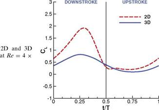 Figure 3.46. Lift coefficient for the (AR = 2) flat plates in shallow stall 104. From Kang et al. [324].
1
|
0.75-
0.25 |
![]()
![]()
![]() 0
0
-1 -0.5 0 0.5 1
x3
1
0.75- 0.25-
0
-1 -0.5 0 0.5 1
xl
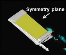
(a) iso-Q-surface at Q = 4 (white) and Q (b) spanwise lift distribution due to pressure. t/T
contours from the 2D computations on the Red dot: 2D; Blue solid: 3D.
symmetry plane.
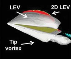
Figure 3.47. Iso-Q surfaces (a) and spanwise lift distribution (b) to illustrate the difference in the flow structures at the center of the downstroke (t/T = 0.25) and the center of upstroke (t/T = 0.75). From Kang et al. [324].
calculated the lift generation on a thin airfoil moving impulsively from rest to a uniform velocity in a 2D incompressible fluid. Vortex wake generated due to the motion of the airfoil affects the force acting on the airfoil. Half of the final lift is generated at the beginning of the motion, and the instantaneous lift asymptotically approaches its final value as a function of increasing time. For harmonically pitching and plunging thin airfoils, Theodorsen [330] derived an expression for the lift by assuming a planar wake and a trailing-edge Kutta condition in incompressible inviscid flow; see Eq. (3-21):
^ _ , nc a h c(2xp — 1)a
Cl (t) = 2П(1 — C{k))a° + ~2 TH + m — 2U2
![]() + 2n C(k) и + a + c(1-5 — 7xv) —
+ 2n C(k) и + a + c(1-5 — 7xv) —
The pitch and plunge motions are described by the complex exponentials, a(t) = a0 + aae(2n ft+V)i andh(t) = hae2n fti. The phase lead of pitch compared to plunge is denoted by f. C(k) is the complex-valued Theodorsen function with magnitude < 1; it accounts for the attenuation of lift amplitude and the time lag in lift response from its real and imaginary parts, respectively. The first term is the steady-state lift, and the second term is the non-circulatory lift due to acceleration effects. The third term models circulatory effects. The same expressions were obtained by Kiissner [331] and von Karman and Sears [332].
For a harmonically plunging thin rigid flat plate in a free-stream, the lift coefficient can be derived assuming inviscid incompressible flow (see Eq. (5-347) as in Bisplinghoff, Ashley, and Halfman [333]):
CL = 2n2St k cos(2n ft) + 4n2 St sin(2n ft), (3-22)
assuming quasi steady-state flow where the influence of the wake vorticities is neglected. The first term in Eq. (3-22) is the non-circulatory term that is consistent with the added mass force derived in Section 3.6.4. The second term in Eq. (3-22) is the circulatory term, which can be expressed in a more familiar form, 2nae, by recognizing that 2nSt sin(2n ft) & ae where ae is the effective AoA for purely plunging motions. Note also that Eq. (3-22) is a simplification of Eq. (3-21) for purely plunging motion with C(k) = 1 equivalent to k ^ 0.
Based on the formulas derived by Theodorsen for the lift and the work by Karman and Burgers [334], Garrick [335] investigated the thrust generation by a harmonically pitching and plunging thin airfoil in uniform free-stream. For a special case of a pure plunge motion the thrust generation CT was
CT = n2 St2 (F2 + G2), (3-23)
where F(k) and G(k) are the real and the imaginary parts, respectively, of the Theodorsen function C(k) – see Eq. (3-21) – predicting greater thrust for higher Strouhal numbers. For a NACA 0012 airfoil Heathcote and Gursul [336] compared the experimentally measured thrust generation with Garrick’s formula [335] and used numerical computation to solve the Navier-Stokes equations [337]. It was shown that Garrick’s formula overestimates the experimentally measured thrust, which is in good agreement with the Navier-Stokes computations.
As discussed in Sections 2.3 and 3.4, the difference between 2D and 3D flow structures in terms of force generation has important implications for the applicability of 2D computations to approximate a 3D flow field. For example, at Re of 102 for a delayed rotation kinematics, the TiV anchored the vortex shed from the leading edge, thereby increasing the lift compared to a 2D computation under the same kinematics (see Section 3.4.1.1). In contrast, under different kinematics with a smaller AoA and synchronized rotation, the generation of TiVs was small, and the aerodynamic loading was captured by the analogous 2D computation (see Section 3.4.1.2). At Re = 0(103-104) Visbal [328] studied the unsteady separation process in a 3D flow field around a purely plunging flat plate with AR = 2, к = 1.0, and St = 0.16. The implicit LES computations employed by Visbal [328] show the evolution of both the TiV and the LEV. The TiV forms as the flat plate plunges downward, breaks down, and collapses during the first part of the upstroke. Meanwhile the LEV, which is fairly uniform at the early stage of downstroke, experiences intense axial flow toward the center of the wing, eventually evolves into an arch-type vortex, and sheds as a ring vortex, suggesting the 3D nature of the flow at higher reduced frequency and Strouhal number.
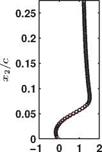
Kang et al. [324] investigated the 3D effects for the flat plate with AR of 2 in shallow stall at Re = 4 x 10⁴. Figure 3.44 illustrates the H1/Um contours from the computations at Re = 4 x 10⁴ and the experimental results obtained at Re = 3 x 10⁴. The flow field is dominated by large leading-edge separation due to the geometric effects in the downstroke as discussed in the previous section. In 3D, the separation is mitigated and the flow reattaches before mid-chord. The velocity field at the center of the downstroke, t/T = 0.25, is further depicted in Figure 3.45 from the 3D computation and experimental measurements at 75 percent span location. The velocity profiles also show the boundary-layer separation at the leading edge and reattachment around xx/cm = 0.25. It should be noted that the experimental measurements were obtained at Re = 3 x 10⁴. The reasonable correlation shown in Figure 3.44 and Figure 3.45 may indicate that the Reynolds number effect is limited, similar to the observation made in Section 3.4.1.2 for the 2D flow around the flat plate.
The absence of the strong leading-edge separation for the flat plate with AR = 2 manifests itself in the aerodynamic force felt on the wing. The time histories of the lift coefficient for both 2D and 3D flat plates in shallow stall are plotted in Figure 3.46. In the upstroke where both flat plates evince attached flow, the lift coefficient shows comparable magnitudes. However, during the downstroke the peak of the lift generated on the 2D flat plate is 2.3 times greater than on its 3D counterpart.
At the center of the downstroke, t/T = 0.25, the effective AoA is at maximum, and the development of the TiV is also significant as illustrated by the iso-surfaces
 |
|||||
|
|
|
|||
|
|
|
||||
|
|||||
 |
|||||
|
|
||||
|
|
|
|||
|
|||||
![]()
Figure 3.45. u1/Uxi profiles at t/T = 0.25 at Re = 4 x 10⁴for the 3D flat plate with AR = 2 in shallow stall at 75% span. Experimental data were performed at Re = 3 x 10⁴. From Kang et al. [324].
of Q in Figure 3.47. This TiV interacts with the LEV developed at the leading edge of the flat plate. Because of the downwash induced from the presence of the TiV, the effective AoA at the leading edge near the tip is smaller than in 2D, which results in a spanwise non-uniform LEV formation that is stronger away from the tip. Consequently, the spanwise lift distribution in 3D is smaller than in 2D as shown in Figure 3.47. Close to the tip of the flat plate a small peak in spanwise lift is shown. A reason for this local maximum is the lower pressure region associated with the presence of the TiV [297]. In contrast, at the center of the upstroke the effective AoA is at minimum, and the flow field has negligible 3D effects such as TiV generation and interactions between TiV and LEV, so that the spanwise lift distribution of 3D is similar to that of 2D.
Figure 3.38 shows the normalized vorticity field around a SD7003 in deep stall, following the same kinematics as introduced in Section 3.5.1 at Re = 6.0 x 10⁴. The phase-averaged field obtained using a 3D implicit filtered large-eddy simulation
 |
xi/c = 0.125 0.25 0.5 0.75 0.25 behind TE
-10 12-1012-1012-1012-1012
Ui/U^l ‘иі/иж ui/U ж ‘иі/иж ui/U ж
t/T= 0.50 (bottom of the downstroke)
Figure 3.36. щ/U^ profiles from the numerical and experimental results at constant x1/cm = 0.125, 0.25, 0.50, 0.75, and 0.25 behind the trailing edge at t/T = 0.00 and 0.50 at Re = 1 x 10⁴ (numerical: dashed line; experimental: square), 3 x 10⁴ (numerical: dash-dotted line; experimental: cross), and 6 x 10⁴ (numerical: solid line; experimental: circle) for the 2D flat plate in shallow stall. From Kang et al. [324].
|
-0.4 x/c |
|
0 |
|
0.25 |
|
0 |
|
0.2 |
(a) implicit LES (b) PIV (c) RANS
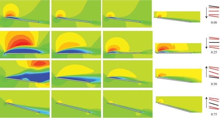
Figure 3.38. Normalized vorticity field around an SD7003 in deep stall. (a) Phase – and spanwise – averaged implicit LES computations by AFRL; (b) phase-averaged PIV measurements by AFRL; (c) RANS computation by University of Michigan. t/T = 0,0.25,0.5, 0.75. From Ol et al. [326].
|
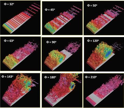
Figure 3.39. Instantaneous iso-Q-surfaces (Q = 500) colored with density showing 3D flow structures at selected phases (Ф) of the motion cycle computed using the implicit LES. From Visbal [327]. |
(LES), phase-averaged PIV, and 2D RANS solutions with Menter’s shear stress transport (SST) turbulence model is included as an example. As the airfoil plunges down, the flow on the suction side starts to separate, forming an LEV. At the bottom of the downstroke, the LEV is already detached, while a well-defined TEV is seen in both computations. A smaller TEV is observed at an earlier phase in the PIV measurements. The smaller details of each vortical structure are well illustrated by the implicit LES computations and the PIV measurements at this Reynolds number. The RANS solution, in contrast, gives a smoother flow field.
The qualitative agreement between the computational and the experimental approaches is better when the flow is largely attached. When the flow exhibits a massive separation (t/T = 0.5), the experimental and computational results show noticeable differences in phase as well as the size of flow separation. Three-dimensional instantaneous flow structures are illustrated in Figure 3.39. The iso-Q-surfaces show the evolution of the vortical structures as computed using an implicit LES solver. At this Reynolds number, the flow during the downstroke and the first part of the upstroke is characterized by three-dimensional small vortical structures that form the LEV, which eventually convects away and breaks down. At the bottom of the downstroke, a well-defined TEV is also clearly visible. Figure 3.40 depicts the lift
 |
 |
Figure 3.40. Time histories of forces on the 2D flat plate (dashed line) and SD7003 airfoil (solid line). From Kang et al. [324].
coefficient computed by the participating institutions for the same case. The upper bound is given by the quasi-steady equation, which is discussed in the next section. The RANS computations result in a smoother lift history than the implicit LES computation, reflecting the vorticity flow field shown in Figure 3.38. Note also that Theodorsen’s lift formula approximates the unsteady lift well (see Section 3.6).
As discussed in the introduction to Section 3.5, Kang et al. [324] investigated the effects of airfoil shapes for the same kinematics, the time histories of force coefficients, and the vorticity contours. Ol et al. [323] discussed in detail the flow physics for SD7003 airfoil at several Reynolds numbers. First, the comparisons of the computed force coefficients are shown in Figure 3.40 for Re = 1 x 10⁴ and 6 x 10⁴ for the flat plate and the SD7003 airfoil. It is clear that the flat plate shows greater lift peaks than the SD7003 airfoil within the range of Reynolds numbers and airfoil kinematics considered in their study [324]. Moreover, Baik et al. [325] observed a phase delay of the peak in the deep stall case at Re = 6 x 10⁴ (see Fig. 3.40b). This is because the flow separates earlier over the flat plate during the downstroke. The corresponding normalized vorticity fields for the SD7003 and flat plate in the deep stall case are shown in Figure 3.41 during the downstroke. The vorticity distribution over the SD7003 airfoil is shown at t/T = 0.33, 0.42, and 0.50 (Fig. 3.41a) and for the flat plate at earlier time instants of t/T = 0.25, 0.33, and 0.42 (Fig. 3.41b). Due to the smaller radius of curvature at the leading edge of the flat plate, the flow around the leading edge experiences a stronger adverse pressure gradient, separating at a lower effective AoA. The leading-edge shear layer and the LEV on the suction side of the flat plate have similar topology to that of the flow field of SD7003 with a phase lag of approximately 0.083. As the LEV and the TEV detach from the airfoils, the difference in lift between these two airfoils diminish.
 |
 |
(c) deep stall, mean (d) deep stall, max
The mean and maximum force coefficients for both airfoil shapes for several Reynolds numbers are summarized in Figure 3.42. The geometric effect due to the sharper leading edge of the flat plate overwhelms the variations in motion kinematics and Reynolds number: the maximum lift is obtained by the flat plate for both kinematics. Furthermore, the force coefficients of the flat plate are insensitive to the Reynolds number. It is also interesting to note that the mean drag coefficient is lower for the SD7003 airfoil because of its streamlined body and that the mean lift coefficient is higher for the SD7003 airfoil for Re = 3 x 10⁴ and 6 x 10⁴, when the flow is attached over most of the motion period.
Sane [312] discussed the effects of delayed stall and LEV on force generation using Polhamus’s analogy [321]. For airfoils without leading-edge separation, the flow over the leading edge accelerates and creates a suction force that is parallel to the chord. This suction force tilts the resulting force forward in the direction of thrust at low AoAs. For a flat plate the flow separates at the leading edge, and an LEV forms on the suction side. The LEV increases the force normal to the flat plate,
I ■
0 0.2 0.4 0.6 0.8 1 1.2 1.4
 |
SD7003 t/T
resulting in increased lift and drag for positive AoA. In this effort, for the shallow stall case, the SD7003 airfoil generates lower lift peak (Fig. 3.40a) but greater thrust compared to the flat plate due to attached flow and leading-edge suction (Fig. 3.40e). Figure 3.43 shows the normalized streamwise velocity contours around the 2D flat plate and the SD7003 airfoil at Re = 6 x 10⁴ for the shallow stall case. During the downstroke the flow separates at the leading edge, forming an LEV that covers the whole suction surface of the flat plate, consistent with the higher lift peak and greater drag during the downstroke shown in Figure 3.40a and Figure 3.40e, while the flow over the SD7003 remains mostly attached. When the prescribed motion is more aggressive for the deep stall case, the flow over the SD7003 airfoil separates near the leading edge during the downstroke (Fig. 3.41), and the resulting lift and drag time histories are similar to those of the flat plate (Fig. 3.40b, f) for the period in which the flow is separated. There is still a significant difference in drag (Fig. 3.40f) during
the first portion of the downstroke, because the flow over the SD7003 airfoil separates later than over the flat plate. Hence, Sane’s application of Polhamus’ analogy is valid for the shallow stall motion and to a lesser extent for the deep stall motion. For motions with greater effective AoA, the flow over the blunt airfoil may separate, and then the resulting force on the blunt airfoil is qualitatively similar to that of a flat plate.
To assess the effects of the Reynolds number on the flow field and the resulting aerodynamic loading, numerical results were obtained for the same kinematics by Kang et al. [324] for Re = 6 x 10⁴, 3 x 10⁴, and 1 x 10⁴. In this Reynolds number range, the Reynolds number sensitivity to the qualitative flow structures is small. This is in contrast to the flows at lower Reynolds number regimes (i. e., O(102)), where the viscosity plays a more important role than at the current Reynolds number, or for the more conventional SD7003 airfoil with a larger radius of curvature at the leading edge [323].
For the deep stall case, Figure 3.35 shows the time history of force coefficients at Re = 1 x 10⁴, 3 x 10⁴, and 6 x 10⁴. Both lift and drag coefficients are negligibly affected by the Reynolds number variation. For all Reynolds number cases, the lift coefficient reaches its maximum near t/T = 0.25, decreases, and starts to increase from t/T = 0.75.
At these moderately high Reynolds numbers, forces due to pressure that arise from large-scale vortical effects, such as LEVs, dominate over viscous forces. The dependence of the small Reynolds number on the u1/Um profiles shown in
|
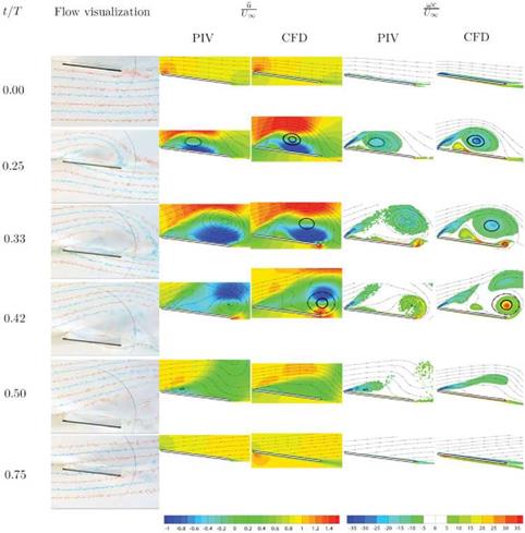
Figure 3.34. Dye injection, u1/UOD and vorticity contours from the flow field around the 2D flat plate in deep stall at Re = 6 x 10⁴ from Kang et al. [324]. |
Figure 3.36 and the qualitative similarity in the large-scale flow features (t/T = 0.50 in Fig. 3.36) suggest that the resulting aerodynamic forces are insensitive to the change in the Reynolds numbers. Figure 3.37 shows the time histories of the force coefficient from the numerical computations. At Re = 1 x 10⁴ the maximum lift coefficient is around t/T = 0.25, which is slightly lower (CL max10K = 1.86) than for Re = 6 x
104 (CL, max, 60K = 1.92) and 3 x 10⁴ (CL, max,30K = 1.90). Simllarly the time histories of the drag coefficient coincide during the downstroke, whereas for Re = 1 x 10⁴ the drag is slightly greater between t/T = 0.50 to 1.00 than at Re = 3 x 10⁴ and 6 x 10⁴.
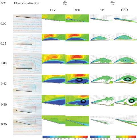
Figure 3.33 shows dye flow visualization, й1/ЦХ!, and m3/(U^/c) contours from Kang et al. [324] for the flow about a flat plate in shallow stall at Re = 6 x 10⁴. They gave the shallow stall kinematics as
h(t/T) = h0cm cos(2nt/T), (3-19)
where h(t/T) is the location of the center of rotation (xp/cm = 0.25) of the airfoil measured normal to the free-stream, h0 = 0.5 is the normalized amplitude of the plunge motion, a(t/T) is the geometrical AoA measured relative to the incoming free – stream with velocity UTO, a0 = 8° is the mean AoA, p = 90° is the phase lag between the pitching and plunging motion, and aa = 8.43° is the amplitude of the pitching motion. The resulting non-dimensional numbers are к = 0.25 and St = 0.08.
As shown in Figure 3.33, leading-edge separation is observed over the majority of the motion cycle. At the top of the downstroke (t/T = 0.00) the boundary layer separates at the leading edge and reattaches before the half-chord, forming a thin shear layer that covers the suction side of the flat plate. As the flat plate plunges down, the effective AoA increases, reaching its maximum at t/T = 0.25. During this portion of the downstroke, the flow field shows flow separation at the leading edge, which produces a closed recirculation region and formation of an LEV capturing the vorticity shed at the leading edge. The LEV is observed during most of the downstroke, convecting downstream, until it eventually detaches from the flat plate at the bottom of the downstroke, t/T = 0.50. A TEV forms at t/T = 0.33, 0.42, and 0.50 due to the interaction of the LEV and the trailing edge. During the upstroke the boundary layer reattaches.
The increase in the induced AoA due to the plunging motion is not compensated by the delayed pitch in the deep stall case where aa = 0° in Eq. (3.20). The flow field is characterized by separated flow throughout the downstroke, consistent with the more aggressive time history of effective AoA [323]. This vortical structure serves as a mechanism to enhance lift by its lower pressure region in the core. Figure 3.34 shows the dye flow visualization, щ/Um, and m3/(U^/c) contours at Re = 6 x 10⁴ from Kang et al. [324]. The LEV is stronger and separates at earlier time instants compared to the shallow stall case. As the flat plate plunges toward the bottom of the downstroke, a well-defined TEV forms at the trailing edge of the flat plate.
Natural flyers such as insects and birds have wings thinner than those of conventional airplanes, such as NACA 0012 or SD7003 airfoils. The effects of kinematics at Re of O(102) in terms of St and к on aerodynamics were discussed in Section 3.4. In this section the effects of airfoil shape on the performance of flapping airfoils at Re of O(104) play a central role in discussing the effects of kinematics, Reynolds number, and 3D as well.
Lentink and Gerritsma [319] investigated numerically the effects of airfoil shape on aerodynamic performance in forward flight. Even though the Reynolds number considered in their study is O(102), they concluded that a plunging thin airfoil with aft camber outperformed other airfoils, including the more conventional airfoil shapes with thick and rounded leading edges. One exception was the plunging N0010 airfoil, which due to its largest frontal area had good performance. At a Reynolds number of 5.0 x 10³, Usherwood and Ellington [320] examined experimentally the effect of airfoil shape of a revolving wing with a planform representative of hawkmoth wings. The results showed that detailed leading-edge shape and airfoil twist and camber do not have a substantial influence on aerodynamic performance.
Sane [312] used Polhamus’s [321] leading-edge suction analogy to explain the lift characteristics of thinner airfoils. The flow around rounded leading-edge airfoils remains attached, creating a leading-edge suction force parallel to the airfoil chord, tilting the resulting aerodynamic force forward toward the incoming flow, and reducing drag. In contrast, flow over an airfoil with a sharp leading edge separates at the leading edge, forming an LEV. The suction force due to the LEV acts normal to the airfoil, increasing both lift and drag. More recently, Ashraf, Young, and Lai [322] numerically investigated the effects of airfoil thickness on combined pitching and plunging airfoils at к = 1 and Reynolds numbers varying from 2.0 x 10² to 2 x 10⁶. They found that at lower Reynolds numbers thin airfoils outperformed thick airfoil, whereas at higher Reynolds numbers the thick airfoil show better performance.
Initiated by the Research Technology Organization (RTO) of NATO, multiple institutions from several countries have investigated the unsteady flow around a pitching and plunging airfoil at Re = O(104) using different methodologies. Ol et al. [323] numerically and experimentally considered the interplay between a SD7003 airfoil undergoing either combined pitching and plunging or purely plunging motions and the resulting aerodynamics at Reynolds numbers 1 x 10⁴, 3 x 10⁴, and 6 x 10⁴ at a fixed Strouhal number and reduced frequency: St = 0.08 and к = 0.25. The two different kinematics produced a shallow stall (under combined pitching-plunging) and a deep stall (under purely plunging) of the instantaneous flow about the airfoil. Kang et al. [324] further reported results on the flow physics of a 2.3 percent thickness flat plate in 2D and 3D configurations and an SD7003 airfoil. In particular, they
|
Figure 3.33. Dye injection, и1/Ц0 and vorticity contours from the flow field around the 2D flat plate in shallow stall at Re = 6 x 10⁴ from Kang et al. [324]. |
showed that due to the small LE radius of curvature of the flat plate, the flow field is dominated by an LEV on the suction side, which could be utilized to manipulate lift production. Furthermore, Sane’s use of Polhamus’s analogy [321] was confirmed for the shallow stall motion.
One of the main difficulties in realizing a functional MAV is its inherent sensitivity to the operating environment because of its size and weight. Wind gusts create intrinsic unsteadiness in the flight environment [318] (see also discussions of the fixed wing in Section 2.2.4) As discussed in Chapter 1, the characteristic flapping time scale of insects and hummingbird – O(10x) to O(102) of Hz – is much shorter than the time scale of a typical wind gust (around O(1) Hz). Hence, from the flapping wing time scale, many wind gust effects can be treated in a quasisteady manner. However, the vehicle control system (as in the case of a biological flyer) operates at lower frequencies, and their time scales are comparable to those of anticipated wind gusts. Therefore, there is a clear multi-scale problem between unsteady aerodynamics, wind gust, and vehicle control dynamics. Since a small bird or insect flaps much faster than commonly experienced wind, the aerodynamics
 |
 |
 70
70
Figure 3.28. Pareto fronts illustrating the competing objectives of time-averaged lift and power requirements in 2D (left) and 3D (right) and the design variable combinations that provide those fronts. The dashed line is for reference.
associated with flapping wings can be pragmatically modeled by a constant free – stream.
Trizila et al. [301] investigated environmental sensitivity in regard to varying kinematic schemes and free-stream strengths and orientations; the same kinematic patterns highlighted in previous sections are adopted again in this discussion. The free-stream strength was fixed at 20 percent of the maximum translational velocity of the wing. Based on parameters associated with fruit flies [Re = O(102) and wing speed is approximately 3.1 m/sec], the free-stream fluctuation would be approximately 0.6 m/s, a relatively light wind gust. The directions of the free-stream varied between heading down, right, or up.
The 2D cases were much more sensitive to the free-stream than their 3D counterparts. Instantaneous lift associated with all three kinematic patterns (synchronized rotation with either low or high AoA and delayed rotation with high AoA) was very sensitive to the horizontal free-stream and much less sensitive to the downward heading free-stream. The downward free-stream generally decreased lift by suppressing vortex generation, while making the forward strokes and backstrokes more symmetric as the vortical activity was washed away from the airfoil more quickly. Overall, the general nature of the force history was kept intact. In contrast, the upwind free – stream had the opposite effect. Namely, the vortex interactions were sustained for a longer period of time, because the free-stream held the wake closer to the airfoil
and the increased AoA also served to accentuate the unsteady aerodynamics. This upward free-stream may or may not have had a significant impact on the force history, which was dependent on the kinematics. The horizontal free-stream had the largest impact over the range of kinematic motions studied, sometimes more than doubling the lift felt for a free-stream strength of 20 percent of the maximum translational velocity, a relatively tame environmental situation leading to a significant change in hovering performance.
Figure 3.29 shows the lift histories and vorticity contours, illustrating the vortex formation and interactions during the LEV-dominated portion of the stroke (Fig. 3.29a-c) and during the wake-capture-dominated portion of the stroke (Fig. 3.29d-f) at their respective maximal lifts for a 20 percent strength headwind hover scenario without free-stream. The 3D LEV-dominated portion of the stroke is highlighted with m3 contours at two spanwise locations with a 20 percent free-stream. Immediately apparent is the large impact on both the instantaneous and time-averaged lift. To clarify, the lift coefficients are still normalized by the velocity related to wing motion (e. g., the mean/maximum translational velocity); that is, the normalization is independent of the free-stream. Flow fields are plotted during the headwind portion of the stroke (backstroke) and show that the headwind case exhibits a more developed and stronger LEV, as well as stronger vorticity shedding from the TE. The increased vortical activity created by the headwind, which then interacts with the airfoil in a favorable manner, qualitatively explains the increase in performance during the backstroke.
However, the significant lift peak in the presence of tailwind is due to a different lift-generation mechanism. This peak occurs after stroke reversal as the airfoil interacts with the previously shed wake, or the wake-capture-dominated portion of the stroke cycle. The hover case temporarily drops off in lift (see Fig. 3.29d), whereas the 20 percent free-stream case, now a tailwind, continues to increase in lift. Vorticity contours at their respective local maximums in lift (see Figs. 3.29e and 3.29f) show a few striking differences, noticeably the strength and position of the previously shed vorticity. The presence of headwind during the backstroke creates stronger vortices. On the return stroke, the strengths of these vortices, in addition to their position relative to the airfoil, significantly help promote vortex growth (see Fig. 3.29f). This interaction, resulting in a temporary enhancement, eventually plays itself out, and a decline in lift ensues in what used to be dominated by the LEV but now amounts to slower relative translational velocity.
Looking at the 2D force histories (Fig. 3.30a) again, one sees that the response of a free-stream depends not only on the kinematics but also on its orientation. Figure 3.31 illustrates the lift response to a free-stream for 2D (Fig. 3.31a-c) and 3D (Fig. 3.31d-f) computations. The free-stream magnitude is 20 percent of the maximum plunging velocity and is headed in three different directions for the three hovering kinematics investigated in the previous two sections (3.4.1.1 and 3.4.1.2). The dotted lines in Figure 3.31a-f are the lift responses of the hovering cases (i. e., no free-stream). For some situations, the qualitative nature of the flow does not change much over the course of the entire cycle, nor are the forces too sensitive; see the vertical free-stream in Figure 3.31a or the downward free-stream in Figure 3.31c. However, the horizontal free-stream has an appreciable impact for all of the kinematic patterns considered in Trizila et al. [301]. Yet the upward and downward
 |
 |
-4 -3.2-2.4-1.6-0.8 0 0.8 1.6 2.4 3.2 4
![]() (j) 2ha = 3.0cm, aa = 45°, and ф = 90°
(j) 2ha = 3.0cm, aa = 45°, and ф = 90°
Figure 3.29. Force history and vorticity contours illustrating the vortex formation and interaction during the LEV dominated portion of the stroke (a-c) or wake capture dominated portion of the stroke (d-f) at their respective maximal lift for a 20% strength headwind free – stream and no free-steam. The 3D LEV-dominated portion of the stroke is highlighted with z-vorticity at two spanwise locations with a 20% free-stream in g, h, and i. Wing motion is shown in j.
 |
|
 |
|
-2.5 -2 -1.5-1 -0.5 0 0.5 1 1.5 2 2.5
x
Figure 3.30. Force history and vorticity contours illustrating the vortex formation between stroke reversal and their respective maximums in lift for (b) 20% downward freestream and (c) 20% upward stream.
free-streams do not necessarily elicit similar responses in opposite directions, as highlighted in Figure 3.30. This brings into question the relevance of using effective AoA in these situations, because the force history may respond more noticeably to the upward free-stream than the downward free-stream; see Figure 3.31a-c, where a 20 percent free-stream imposed from different directions significantly changes the qualitative behavior of the resulting force history.
For all of the synchronized rotation cases (which have positive AoAs at all times), a 20 percent downward free-stream does indeed decrease the lift. The downward free-stream also suppresses the vortical flow strength as the effective AoA is lowered. However, some cases have a much more pronounced sensitivity to the upward free – stream. Figure 3.30a illustrates again the force histories for a 20 percent free-stream at various orientations relative to the hover case, as well as the vorticity flow field (Figs. 3.31a and 3.31c) for the 20 percent upward and downward free-stream cases at a time where the difference in force history between the two is pronounced. What is seen in Figure 3.30b and Figure 3.30c is the increase in LEV and TEV formation, as well as a more pronounced interaction with the wake, as the upward free-stream promotes the growth of the vortex structures and holds the wake in the vicinity for a longer period of time. The non-linear response in lift as the free-stream lowers or raises the effective AoA is a product of these factors.
The 3D cases, in contrast, are much less sensitive to the free-stream (see Fig. 3.29 g-i and Fig. 3.31 d-f. Note, however, that the scale for the force histories was chosen so that they could be directly compared with the 2D case and the free – stream could be quite influential. The impact is non-negligible for a 20 percent strength free-stream, but overall, the nature of the flow is very similar for most cases.
Figure 3.31. 2D (a-c) and 3D (d-f) CL in response to a free-stream with a
The downward free-stream once again degrades lift, and the upwind free-stream enhances it, albeit to a lesser degree than in the 2D cases.
Figure 3.32 highlights the vortex interactions at the beginning, middle, and ending of the strokes for a 20 percent free-stream tailwind. The blue arrow in vorticity contours for 2D and at mid-span and the wingtips for 3D denote free-stream directions. The 3D wing is unable to generate vortices of the same magnitude as the analogous 2D counterpart. This inability directly affects the wing’s benefit from LEV interactions, as well as subsequent interactions with the previously shed wake. The spanwise variation of vorticity exhibited shows a decrease in LEV generation from mid-span to tip, and although the tip vortices are prominent, they do not make up for the weakened LEV formation and wake interaction, as experienced in 2D. Figure 3.29 illustrates the vorticity flow fields during maximal lift during the headwind, resulting in a 2D lift (Fig. 3.29a) that is almost twice as large as its 3D counterpart (Fig. 3.29g).
 |
This discrepancy in sensitivity to free-stream between 2D and 3D shows up across the range of kinematic motions. A limited subset of kinematic motions show very similar force histories in the time-averaged sense, as well as instantaneously (see Section 3.4.1.2) when not under the influence of an external free-stream. The kinematics in this region of the design space shares low AoAs across much of the flapping cycle and synchronized rotation, limiting the high angular velocities. A lower angular velocity, in turn, tends to limit vortex size, strength, formation, and influence. As the free-stream is introduced (see Figs. 3.31c and 3.31f for 2D and 3D force histories, respectively, in the presence of a 20 percent free-stream), the response is not uniform across the span of the finite wing. The downward free-stream (20 percent strength) tends to suppress the vortex dynamics, and as such, the 2D
and 3D force histories remain quite similar. In contrast, the horizontal free-stream, most notably during the headwind and the upward free-stream, shows differences due to the 3D nature of the flow; the reader is referred to Trizila et al. [315] for more details, which include further flow field examinations not described here for the sake of conciseness.
In a multi-objective investigation, it is often the case that different goals are in competition when selecting design variables. One tool used to evaluate the tradeoffs between objective functions is called the Pareto front [317], which consists of non-dominated points and can be thought of as the set of best possibilities. Non – dominated points are those points for which one could not improve all objective functions simultaneously.
Trizila et al. [301] presented the Pareto front for the competing objectives of maximizing time-averaged lift and minimizing the power requirement in the 2D and 3D hovering flat plate case highlighted in previous sections, as illustrated in Figure 3.28. Points on the Pareto front therefore involve those for which increases in lift are accompanied by increases in power, and vice versa. The resulting Pareto front itself is very comparable between 2D and 3D (see Fig. 3.28). The primary differences are that the peak lift values attained in 2D exceed their 3D counterparts and the density of the design variable combinations near the Pareto front is higher in the 3D case. The paths through the design space are plotted below their respective Pareto fronts in Figure 3.28. Note that the jaggedness of the path is due to the resolution of the tested points and the fine balance in objective functions for design variables in that region. The high-lift region follows the lower bound of the angular amplitude, suggesting that future iterations should decrease the lower bound for higher lift solutions. Overall, the design variable combinations on the optimal front are consistent qualitatively. The high time-averaged lift values are obtained by a combination of advanced rotation and low angular amplitude in the 2D and 3D cases. The general trends remain largely the same.
There are interesting combinations of wing kinematics that result in similar lift in both 2D and 3D. For some cases, even the instantaneous forces agree well.
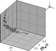
Figure 3.27 shows the flow fields of such a case corresponding to these kinematic parameters: 2ha = 3.0cm, aa = 80°, and у = 90° at t/T = 0.8, 1.0, and 1.2. The variation along the spanwise direction is modest, making the 2D and 3D simulations substantially similar. The 2D flow field and the corresponding 3D flow on the symmetry plane are strikingly consistent. The high angular amplitudes lead to low AoAs
Figure 3.26. Force history (2D: red, 3D: black) for a motion cycle and z-vorticity contour plots at three time instants in the forward stroke for the delayed rotation and low AoA (2ha = 4.0cm, aa = 80°, and <p = 60°): (a) from 2D computation; (b) in the symmetry plane of 3D computation; (c) near the wingtip (z/c = 1.8) plane.
 |
and, coupled with the timing of the rotation, lead to a flow that does not experience delayed stall, because the formation of LEVs is not promoted. The timing of the rotation for this example puts the flat plate at its minimum AoA (10°) at the moment of maximum translational velocity, while the translational velocity is zero when the flat plate is vertical. It is seen from the flow field that both the TiV and the LE/TE vortex formation are largely suppressed. The net effect is a fairly uniform spanwise lift distribution, closely resembling the 2D case with the same kinematics.
Neither the 2D nor 3D results in this case promote downward induced jet formation. As summarized in Figure 3.27, the 2D and 3D lift coefficients are similar in the instantaneous and time-averaged senses. One implication of this similarity is the usefulness of the 2D simulation for generating quantitative data on a 3D counterpart. However, not all cases in this region display this similar instantaneous behavior, and sometimes the time-averaged lift similarity results from the partial canceling out of different features.
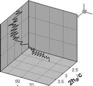
SYNCHRONIZED HOVERING, HIGH AOA – PRESENCE OF A PERSISTENT JET. As shown in region 1 in Figure 3.21d, the kinematics in this region corresponds to nearly synchronized hovering (i. e., including cases with slightly delayed or advanced rotation), low angular amplitude (high AoA), and larger plunging amplitudes. Figure 3.22 shows the time history of lift and vertical velocity contour plots at three time instants: in the forward stroke from the 2D simulation, in the symmetry plane of the 3D computation, and near the wingtip. It can be seen that there are two local maxima per stroke in 2D. The first peak is associated with the wake capture at the beginning of the
![]()
 |
 |
Figure 3.22. Instantaneous force history (2D: solid, red; 3D: broken, black) and vertical velocity contour plots at three time instants in the forward stroke for the synchronized rotation and high AoA (2ha = 3.0cm, aa = 45°, and <p = 90°): (a) 2D computation; (b) in the symmetry plane of 3D computation; (c) near the wing tip (z/c = 1.8).
stroke at t/T = 0.8. Between the two peaks, there is a local minimum referred to as a “wake” valley, which is caused by a combination of decreasing AoA and interaction with a pocket of downward momentum that takes the form of a persistent jet. As reported during the experimental studies of Freymuth [175], the jet develops as a result of a reverse Karman vortex street interacting with the downward momentum created by the wing as it translates. As the wing passes the jet, vortices are shed with an orientation that reinforces the downward momentum previously created by
 |
 |
-2-10 1 2 3
x
U2
Figure 3.23. Time history of lift coefficients in a representative case in region 2; the advance rotation and low AoA (2ha = 4.0cm, aa = 80°, and <p = 120°), with the associated flow features. (a) Lift, (CL), during a motion cycle. Red-solid, 2D computation; black-dashed, 3D computation. (b) Kinematic schema of the flat plate motion. (c) Representative flow features at (1) t/T = 0.9, vertical velocity (u2) contours; (2) t/T = 1.0, vorticity contours; (3) t/T = 1.2, vertical velocity contour.
the wing. These vortices sustain the downward momentum, and they further entrain surrounding fluid to create a flow feature with which the wing then interacts during subsequent strokes. In 3D, the weaker downward momentum pocket does help generate lift compared with 2D, which can be confirmed in the instantaneous lift history at t/T = 0.9. In 2D, the persistent jet shows larger vertical velocity magnitude and is narrower. However, the weaker LEV has a negative effect on the lift. In the 2D case, the LEV is largely attached, and anchoring the LEV has no benefit. Overall, for this case, the 2D lift is better than the 3D counterpart. More generally, cases in region 1 as shown in Figure 3.21d have larger lift in 2D.
advanced rotation and low aoa – higher 3D lift. In region 2 as shown in Figure 3.21d, the kinematics is characterized by advanced rotation and a high angular amplitude. Figure 3.23 shows the time histories of lift and the associated flow
features for an advanced rotation case with a generally low AoA (2ha = 4.0cm, aa = 80°, and p = 120°). Right after the stroke reversal, the flat plate moves into the wake generated in the previous stroke. Because of the downwash in this wake (see also Fig. 3.23) and the low and decreasing AoA (Fig. 3.23b), lift drops. Note that the pocket of downward momentum encountered for these kinematics is not a persistent jet: the 3D case does not suffer the same drop in lift as the 2D case.
DELAYED ROTATION AND HIGH AOA – TIP VORTEX CAN ENHANCE LIFT. Region 3 is defined by the kinematics with delayed rotation, low angular amplitude (high AoA), and shorter plunging amplitudes. This region shows a significant impact from the TiVs. Figure 3.24 illustrates a delayed rotation case with high AoA (2ha = 2.0cm, aa = 45°, and p = 60°). The difference in the flow physics encountered due to 3D phenomena is noticeable. The main characteristics of the vortices, including their sizes, strengths, and movement, are distinctly different between 2D and 3D results. Not only is there a strong spanwise variation in the 3D flow but there is also little resemblance between the symmetry plane of the 3D and the 2D computations.
In 2D flow the pair of the large-scale vortices is noticeably closer to each other and the airfoil than in the 3D flow. The instantaneous lift coefficient for the two cases examined is illustrated in Figure 3.24; the 3D lift coefficient is generally higher than its 2D counterpart. With these kinematics patterns, the TiVs can interact with the LEV to form a lift-enhancement mechanism. This aspect is discussed next.
Figure 3.25 shows an iso-Q contour colored by rn3, the spanwise vorticity in forward stroke. In this fashion we can separate the rotation from the shear, via Q, which can be used as a measure of rotation; we can then obtain directional information with vorticity. The vortices shed from the leading and trailing edges are identified by red and blue colors, respectively, whereas the TiV is green. The role of the TiV in the hovering cases studied is particularly interesting. For the case presented in Figure 3.25 (delayed rotation) – the Q iso-surface colored with «3-vorticity, along with the spanwise distribution of CL due to pressure – the effects of the tip vortices become apparent. First, a low-pressure region at the wingtip favorably influences the lift. Second, the TiV anchors the large-scale vortex pair near the tip. At mid-span, however, the vortex pair has separated from the wing. This in turn drives the spanwise variation seen in the flow structures and force history.
Compared with an infinite wing, the TiVs cause additional mass flux across the span of a low-aspect-ratio wing, which helps push the shed vortex pair, from the leading edges and trailing edges, at mid-span away from one another. Furthermore, there is a spanwise variation in effective AoA induced by the downwash, which is stronger near the tip. Overall, the TiVs allow the vortex pair in their neighborhood of the tip to be anchored near the wing surface, which promotes a low-pressure region and enhances lift. The end result is an integrated lift value that departs considerably from the 2D value.
From the discussions in this section, it is clear that the kinematic motions have a significant impact on TiV formation and LEV/TEV dynamics. Interestingly, for many of the kinematic motions examined, the TiV force enhancement could be confined to lift benefits; that is, the resulting drag did not increase proportionally.
 |
|
Figure 3.24. Force history (2D: solid red, 3D: dash black) for a flapping cycle and z-vorticity contour plots at three time instants in the forward stroke for the delayed rotation and high AoA (2ha = 2.0cm, aa = 45°, and <p = 60°): (a) 2D computation; (b) in the symmetry plane of 3D computation; (c) near the wingtip (z/c = 1.8).
DELAYED ROTATION, LOW AOA, LOW AMPLITUDE – ABSENCE OF WAKE CAPTURE IN 3D.
The kinematics in region 4 is characterized by delayed rotation, large angular amplitude (or low AoA), and shorter plunging amplitude (see Fig. 3.21d). Note that the phase lag between the plunging and pitching motion is similar to that of previous sections, but the amplitude of both pitch and plunge differs. Figure 3.26 shows the time histories of lift from the 2D and the 3D computations, along with a schema for the kinematics as a representative case for region 4: 2ha = 2.0cm, aa = 80°, and = 60°. The largest discrepancy between 2D and 3D is seen around t/T = 0.9. Because the rotation is delayed, after the stroke reversal at t/T = 0.75 the flat plate creates rotational starting vortices to increase the lift, with its first peaks around t/T = 0.9. However, as shown in Figure 3.26, in the 2D case, the TEV shed in
the previous stroke interacts with the flat plate after the stroke reversal, thereby enhancing the lift by the wake-capture mechanism (t/T = 0.9). In contrast, for the 3D case, the shed LEV and the TEV repel from each other and from the path of the flat plate, such that after the stroke reversal, the wake capturing is absent. The first lift peak in the time history in Figure 3.26 is then only due to the rotational effects. So the diverging behavior of the vortices, observed for all delayed rotation cases, and the interaction of the vortices from the leading and trailing edges with the TiVs, play a central role as important 3D effects as described in the previous section.