Our heavyweight helicopter equal in the world does not have
In Rostov started production of the most load-lifting rotary-wing car The Russian holding «Helicopt[...]

Everything about aircrafts and helicopters. News and events in aviation worldwide. Civil, transportation, military helicopters and airplanes.

Everything about aircrafts and helicopters. News and events in aviation worldwide. Civil, transportation, military helicopters and airplanes.

Everything about aircrafts and helicopters. News and events in aviation worldwide. Civil, transportation, military helicopters and airplanes.

Everything about aircrafts and helicopters. News and events in aviation worldwide. Civil, transportation, military helicopters and airplanes.


3.4.1 Effects of Kinematics on Hovering Airfoil Performance
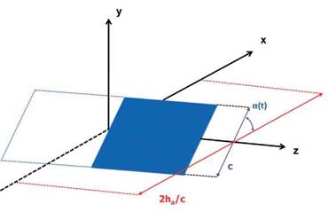
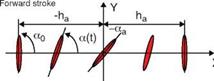
Trizila et al. [301] used surrogate modeling techniques [314] to investigate the time – averaged lift and power input subject to various combinations of kinematic parameters and reported numerous interesting findings. They considered a 2 percent thick wing with AR = 4. The Reynolds number, based on the average tip velocity, is equal to 64, which is similar to that of a fruit fly, Drosophila melanogaster. They used simplified wing kinematics (see Eqs. (3-4) and (3-5)) and selected the mid-chord of the rigid airfoil as the pitching axis. Because the free-stream is absent, the tip velocity is taken as the reference velocity, so that the reduced frequency contains the same information as the inversed normalized stroke amplitude [315]. The rotational (pitching) motion is similarly governed by the flapping frequency, and the angular amplitude, aa, is a measure of how far the airfoil deviates from the yz-plane (see Fig. 3.20). The time average of the pitching motion is a0 = 90°. Higher angular amplitudes yield lower angles of attack and vice versa. The phase lag between the pitching and plunging motions is denoted as q>.
The three kinematic parameters used as the design variables in surrogate modeling – stroke amplitude (ha), pitching angular amplitude (aa), and phase lag (<p>) – are varied independently. The range of the design variables is as follows. The normalized stroke amplitude is representative of a range of flapping wing flyers: 2.0 < 2ha/cm < 4.0. Details on pitch amplitude and phase lag are not as plentiful in the literature, so cases are chosen with low AoAs (amin = 10°; high pitching amplitude) and high AoAs (amin = 45°; low pitching amplitude): 45° < aa < 80°. The bounds on phase lag are chosen to be symmetric about the synchronized hovering: 60° < < 120°. Although delayed rotation is not a focus of many studies found in the
![]()
|
|
|
|
|
|
|||
 |
|||
|
|||
|
|||
|
|
||
|
|
||
|
|||
|
|||
|
|||
|
|||
|
|||
|
|||
![]()
(c) (d)
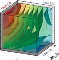
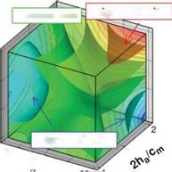
Figure 3.21. Iso-sufaces of 2D lift (a), 3D lift (b), 3D minus 2D lift (c), and (d) where the absolute difference between the 2D and 3D lift equals 0.10. The symbols denote training points in those regions for which detailed force histories and flow field quantities are available; brown octahedra (region 1), circles (region 2), black quarter sphere (region 3), and a blue cube (region 4). The blue region in (c) denotes kinematics for which the 2D lift is higher than the equivalent 3D kinematics. Likewise the yellow/red region denotes higher 3D time-averaged lift.
literature because of the lift-lowering rotational effects, the delayed rotation cases offer interesting wake interactions in 3D.
The quantities of interest – the objective functions in the surrogate modeling nomenclature – are the time-averaged lift coefficient and an approximation of the power required over the stroke cycle. Furthermore, based on the guidance from the surrogate models, Trizila et al. [301] probed the fluid physics associated with 2D and 3D cases and were able to highlight the effects of wing kinematics on hovering airfoil performance. The impact on lift from the 2D/3D unsteady mechanisms including interactions between the LEV and TiVs is detailed in subsequent sections.
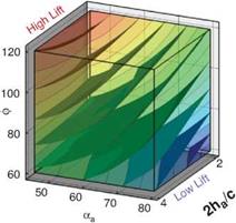
Figure 3.21 shows the iso-surfaces of the time-averaged lift coefficient where each axis corresponds to one of the kinematic parameters (i. e., ha, aa, or <p). Figure 3.21a-c
correspond to the 2D lift, 3D lift, and the difference between the two, respectively. Observations that are immediately apparent are that kinematic combinations with a low aa (high AoA) and advanced rotation (high ф) have the highest mean lift in 2D and 3D. This result qualitatively agrees with the results of Wang et al. [217] and Sane and Dickinson [292]. Due to the non-monotonic response in phase lag (ф) found in the 2D lift response at high pitching amplitudes (see Fig. 3.21a), there are two regions where there is low, and possibly negative, time-averaged lift generation. The first region is defined by low plunge amplitudes (low 2ha/cm), low AoA (high aa), and advanced rotation (high ф). The second region is defined by low AoA (high aa), and delayed rotation (low ф) and is where the 3D kinematics also generates low time-averaged lift values.
A variable’s sensitivity is directly related to the gradients along the respective design variables, whereas a more quantitative measure is the global sensitivity analysis; these measures were examined in Trizila et al. [301]. The gradients along the aa and ф axes are much more significant than that along the normalized stroke amplitude. (Note: Lua et al. [316] found that the effect of Re is noticeably smaller than that of aa on the mean lift.) Furthermore, Figure 3.21 shows that advancing the phase lag is beneficial in 2D except when at high aa; in 3D there is no such exception within the bounds studied. Comparisons with Sane and Dickinson’s experiments [292] show qualitative agreement in the trends in time-averaged lift as a function of aa and ф within the common ranges, with the noticeable difference in setups being one study [301] used pure translation to represent the plunge whereas the experimental study flapped about a pivot point.
The difference between 2D and 3D time-averaged lift may raise a question about areas of the design space for which simplified 2D aerodynamic analyses can sufficiently approximate their analogous 3D counterparts versus those areas where there are substantial 3D effects, which would preclude such a comparison. Figure 3.21c suggests that the difference in the time-averaged lift coefficient larger than 0.1 is due to three-dimensionality.
Following Shyy et al. [296] and Trizila et al. [301], we now highlight four cases corresponding to those presented in Figure 3.21: (i) synchronized hovering, high AoA; (ii) advanced rotation, low AoA; (iii) delayed rotation, high AoA, low plunging amplitude; and (iv) delayed rotation, low AoA, and low plunging amplitude. Each of these cases represent a region where the lift for the low AR wing is significantly different in 2D than in 3D, as indicated in Figure 3.21. In addition to these cases, we look at another region where 2D lift is similar to 3D lift and discuss the trade-off between lift and power.
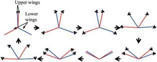
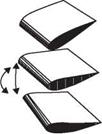
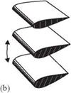
One of the most complex kinematic maneuvers in flying animals is the wing-wing interaction of the left and right wings during the dorsal stroke reversal, termed the clap-and-fling mechanism (see Fig. 3.17). This unique procedure enhances lift generation and is particularly observed in the flight of tiny insects [68]. It has been further observed in other studies [70] [303] [304]. A modified kinematics termed “clap-and-peel” was found in tethered flying Drosophila [305] and larger insects such as butterflies [26], the bush cricket, mantis [306], and locust [307]. It seems that the clap-and-fling mechanism is not used continuously during flight and is more often
|
Clap |
|
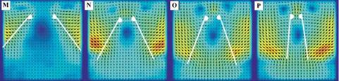
Fling Figure 3.18. Experimental visualization of clap-and-fling mechanism by two wings (M-T) using robotic wing models; from Lehmann et al. [273]. Vorticity is plotted according to the pseudo-color code, and arrows indicate the magnitude of fluid velocity, with longer arrows signifying larger velocities. |
observed in insects during maximum flying performance while carrying loads [308] or performing power-demanding flight turns [307]. Marden’s experiments [308] on various insect species found that insects with the clap-and-fling wing-beat produce about 25 percent more lift per unit flight muscle (79.2 N kg-1mean value) than insects using conventional wing kinematics (such as flies, bugs, the mantis, dragonflies, bees, wasps, beetles, and sphinx moths; 59.4 N kg-1mean value).
The clap-and-fling mechanism is a close apposition of two wings at the dorsal stroke that reverses preceding pronation. By strengthening the circulation during the downstroke it can generate considerably large lift on the wings. The fling phase preceding the downstroke is thought to enhance circulation due to fluid inhalation in the cleft formed by the moving wings, which causes strong vortex generation at the leading edge. Lighthill [209] showed that a circulation proportional to the angular velocity of the fling was generated. Maxworthy [43], by a flow visualization experiment on a pair of wings, reported that during the fling process, an LEV is generated on each wing and its circulation is substantially larger than that calculated by Lighthill [209].
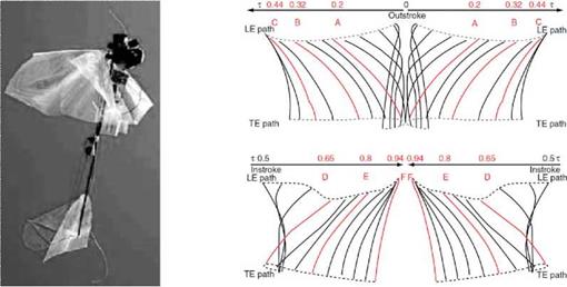
Lehmann et al. [273] used a dynamically scaled mechanical model fruit fly Drosophila melanogaster wing to investigate force enhancement due to contralateral wing interactions during stroke reversal (clap-and-fling; see Fig. 3.18). Their results suggest that lift enhancement during clap-and-fling requires an angular separation between the two wings of no more than 10°-12°. Within the limitations of the robotic apparatus, the clap-and-fling augmented the total lift production by up to 17 percent, but the actual performance depended strongly on stroke kinematics. They measured two transient peaks of both lift and drag enhancement during the fling phase: a prominent peak during the initial phase of the fling motion, which accounts for most
of the benefit in lift production, and a smaller peak of force enhancement at the end of the fling when the wings started to move apart. Their investigation indicates that the effect of clap-and-fling is not restricted to the dorsal part of the stroke cycle but that it extends to the beginning of the upstroke. This suggests that the presence of the image wing distorts the gross wake structure throughout the stroke cycle.
Recently, Kolomenskiu et al. [309] investigated the clap-fling-sweep mechanism of hovering insects using 2D and 3D simulations at specific Reynolds numbers: 1.28 x 10² and 1.4 x 10³. The results showed that the 3D flow structures at the beginning of the downstroke are in reasonable agreement with the 2D approximations. After the wings move farther than one chord length apart, the 3D effects can be seen in force history and flow structures for both Reynolds numbers. At Re = 1.28 x 10², the spanwise flow from the wing roots to the wingtips is driven by the centrifugal forces acting on the mass of the fluid trapped in the recirculation bubble behind the wings. The spanwise flow removes the excess of vorticity and delays the periodic vortex shedding. At Re = 1.4 x 10³, vortex breakdown occurs past the outer portion of the wings, and multiple vortex filaments are shed into the wake.
This clap-and-fling mechanism is being applied to enhance lift of actual flapping wing MAVs (de Croon et al. [310] and Nakata et al. [311]; see Figure 3.19).
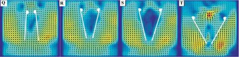
Tip vortices (TiVs) associated with fixed finite wings are seen to decrease lift and induce drag [297]. However, in unsteady flows, TiVs can influence the total force exerted on the wing in three ways: (i) by creating a low-pressure area near the wingtip [296], (ii) through an interaction between the LEV and the TiV [296], and (iii) constructing a wake structure by downward and radial movement of the root vortex and TiV [298]. The first two mechanisms (see Fig. 3.15) also were observed for impulsively started flat plates normal to the motion with low aspect ratios: Ringuette et al. [299] presented experimentally that the TiVs contributed substantially to the overall plate force by interacting with the LEVs at Re = 3.0 x 10³. Taira and Colonius [300] used the immersed boundary method to highlight the 3D separated flow and vortex dynamics for a number of low aspect ratio flat plates at different AoAs. At Reynolds numbers of 3.0 x 10² to 5.0 x 10², they showed that the TiVs could stabilize the flow and exhibited non-linear interaction with the shed vortices. Stronger
 |
 |
influence of the downwash from the TiVs resulted in reduced lift for lower aspect ratio plates.
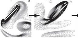
For flapping motion in hover, however, depending on the specific kinematics, the TiVs could either promote or make little impact on the aerodynamics of a low aspect ratio flapping wing. Shyy et al. [296] demonstrated that for a flat plate with AR = 4 at Re = 64 with two different wing motions (such as delayed rotation and synchronized rotation; see Fig. 3.16), the TiV anchored the vortex shed from the leading edge, thereby increasing the lift compared to a 2D computation under the same kinematics. In contrast, under different kinematics with a small AoA and synchronized rotation, the generation of TiVs was small, and the aerodynamic loading was well approximated by the analogous 2D computation. They concluded that the TiVs could either promote or make little impact on the aerodynamics of a low aspect ratio flapping wing by varying the kinematic motions [296]. Furthermore, at Re = 64, Trizila et al. [301] found that four prominent competing effects were in play due to TiVs:
1. Enhancement of lift due to the proximity of the associated low- pressure region
of the tip vortex next to the airfoil
 |
 |
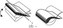
Figure 3.17. Sectional schematic of wings approaching each other to clap (a-c) and fling apart (d-f), from Sane [312] and originally described in Weis-Fogh [68]. Black lines show flow lines and dark blue arrows show induced velocity. Light blue arrows show net forces acting on the airfoil. (a-c) Clap. As the wings approach each other dorsally (a), their leading edges touch initially (b), and the wing rotates around the leading edge. As the trailing edges approach each other, vorticity shed from the trailing edge rolls up in the form of stopping vortices (c), which dissipate into the wake. The leading-edge vortices also lose strength. The closing gap between the two wings pushes fluid out, giving an additional thrust. (d-f) Fling. The wings fling apart by rotating around the trailing edge (d). The leading edge translates away and fluid rushes in to fill the gap between the two wing sections, giving an initial boost in circulation around the wing system (e). (f) A leading edge vortex forms anew, but the trailing-edge starting vortices are mutually annihilated because they are of opposite circulation.
2. Induced downwash acting to reduce the effective AoA along the span and weakening the LEV, hence reducing the instantaneous lift
3. Interaction with the vortices shed from the LEs and TEs and anchoring them from shedding near the wingtips, thereby enhancing the lift
4. Because TiVs pull fluid from the underside of the wing to the upper side, the wing leaves behind a weaker pocket of downward momentum in the flow. On interaction with this downward momentum, a loss in lift is seen, and so a weaker wake valley means higher lift.
As discussed by Dickinson et al. [201] the wing-wake interaction can significantly contribute to lift production in hovering insects. They found that the second peak is generated at the beginning of each stroke of hovering flight when the wings reverse the direction of moving while rotating about the spanwise direction. This physical mechanism, termed wake capture, produces aerodynamic lift by transferring fluid momentum to the wing at the beginning of each half-stroke. A wing meets the wake created during the previous stroke after reversing its direction, thus increasing the effective flow speed surrounding the airfoil, which generates the second force peak. The wake-capture mechanism is illustrated in Figure 3.14.
As with rapid pitch-up, the effectiveness of wake capture is a function of wing kinematics and flow structure. This second force peak (occurring right after stroke reversal) is apparently distinct from rotational lift because its timing is independent of the phase of wing rotation. Dickinson et al. [201] showed that the second peak persists even by halting the wing after it rotates, indicating that the wake produced by the wing motion in the previous half-stroke serves as an energy source for lift production.
The sinusoidal motion along a horizontal stroke plane is similar to that shown by Wang et al. [217], who conducted 2D simulation of a hovering elliptic airfoil with the stroke amplitude ha between 1.4c and 2.4c, leading to a reduced frequency (Eq. (3-11)) k between 0.36 and 0.21. The Reynolds number considered is between 75 and 115. The computational results of Wang et al. [217] and Tang et al. [244] both identify a lift peak after the stroke reversal for the normal hovering mode (see Fig. 3.7). However, for the “water treading” mode, the results of Tang et al. [244] show a continuous increase in lift as the airfoil pitch angle increases to its maximum value without a noticeable peak. More detailed discussion of the lift generation for both normal and water treading hovering modes can be found in Tang et al. [244].
|
T T Figure 3.15. Drag coefficients of AR 6 and 2 flat plates during a starting-up translation as a function of T (the number of chord lengths the plate has traveled, see definition of [302]), from Ringuette et al. [299]. (a) Overall view; (b) detailed view of (a). Both (a) and (b) show drag coefficients for the free tip AR of 6 plate (continuous line) and for the same plate with the tip grazing a raised bottom (dash-dotted line); the dashed line is drag coefficient for the AR of 2 plate with the tip free. Low AR of the wing reduces the drag coefficient significantly due to interactions between a TiV and a LEV. |
This interpretation of wake-capture force generation has been questioned recently based on the claim that the rotation-independent lift peak is due to a reaction caused by accelerating the added mass of fluid [293]. In general, the inertia of the flapping wing is increased by the mass of the accelerated fluid – termed added mass [45] – which can play a significant role in the aerodynamics of insect flight [294]. However, evaluating the added mass, and thus estimating inertial forces, is, not easy. Although the mass of a wing itself may be tiny, the mass of the accelerated fluid need not be [65] [295].
The LEV-based lift-enhancement mechanism seems to be a main feature during the translational motion of the stroke. In addition, the flapping wings experience rapid wing rotation at the ends of the down – and upstroke, which can enhance lift force in flying insects.
Kramer [288] first demonstrated that a wing can experience lift coefficients above the steady stall value when that wing is rotating from low to high AoAs, which is now termed the Kramer effect. The unsteady aerodynamic characteristics associated with the time-dependent AoA, including hysteresis, are shown in Figure 3.4. Dickinson et al. [201] used their Robofly along with a varied rotational pattern, illustrated in Figure 3.9, to investigate the interplay between kinematics and lift generation. They identified two aerodynamic force peaks at the end and the beginning of each
 stroke (pronation and supination). The first force peak can be explained based on the rotational circulation. The resulting force enhancement is influenced by the timing of the wing rotation while translating. They found that an advanced rotation produces a mean lift coefficient CL = 1.74, which is almost 1.7 times higher than that of a delayed rotation (CL = 1.01), whereas a symmetric rotation can attain a value of CL = 1.67. These peaks were confirmed by the numerical simulations of Sun and Tang [289] and Ramamurti and Sandberg [290]. In addition, Sun and Tang [291] further investigated three mechanisms responsible for lift enhancement via unsteady aerodynamics: (i) rapid acceleration of the wing at the beginning of a stroke, (ii) delayed stall, and (iii) fast pitch-up rotation of the wing near the end of the stroke. In advanced rotation, the wing flips before reversing its translational direction as illustrated in Figure 3.9, and the leading edge rotates backward relative to the translation. Based on their computational analysis, Sun and Tang [289] suggested that the first peak is due to the increase in rapid vorticity that occurs when the wing experiences fast pitch-up rotation. The pitch-up rotation and the associated vorticity increase are plotted in Figure 3.13f and g. Sane and Dickinson [292] attributed this first force peak to the additional circulation generated to reestablish the Kutta condition during the rotation. Overall, the findings reported by Sun and Tang [289] and Sane and Dickinson [292] are in agreement. The second peak, termed wake capture, is related to the wing-wake interaction and is discussed next. Together, these two peaks contribute to lift enhancement. Because both pitch-up and wake
 ‘V
‘V
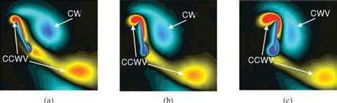
![]() Figure 3.14. Illustrations of the wake-capture mechanism [201] [296]. (a) Supination, (b) beginning of upstroke, and (c) early of upstroke. At the end of the stroke, (a), the wake shed in the previous stroke denoted by CWV is en route of the flat plate. As the flat plate moves into the wake (b-c) the effective flow velocity increases and additional aerodynamic force is generated. The color of the contour indicates the spanwise component of vorticity. CWV and CCWV indicate clockwise and counterclockwise vortex.
Figure 3.14. Illustrations of the wake-capture mechanism [201] [296]. (a) Supination, (b) beginning of upstroke, and (c) early of upstroke. At the end of the stroke, (a), the wake shed in the previous stroke denoted by CWV is en route of the flat plate. As the flat plate moves into the wake (b-c) the effective flow velocity increases and additional aerodynamic force is generated. The color of the contour indicates the spanwise component of vorticity. CWV and CCWV indicate clockwise and counterclockwise vortex.
capture are strongly influenced by flapping kinematics, more discussion is provided later to help elucidate the parametric variations of these factors.
When an airfoil is accelerated impulsively to a constant velocity, the bound vortex needs time to develop to its final, steady-state strength. Depending on the pace of acceleration, it may take up to six chord lengths of travel for the circulation and lift to reach 90 percent of the final values [213]. This lift enhancement can be explained in part by the so-called Wagner effect [274], which describes the unsteady aerodynamics associated with an accelerating airfoil. Specifically, an impulsively started airfoil only develops a fraction of its steady-state circulation immediately; the steady-state value can be attained only after the airfoil moves through several chord lengths. However, if the airfoil is started at an AoA above its stalling angle, then a large transient vortex forms above the leading edge, which can dramatically increase the lift [51]. Dickinson and Gotz [275] measured the aerodynamic forces of an airfoil impulsively started at a high AoA in the Reynolds number range of a fruit fly (Re = 75-225). They
observed that, at AoAs above 13.5°, impulsive movement resulted in the production of an LEV that stayed attached to the wing for the first two chord lengths of travel, resulting in an 80 percent increase in lift compared with the performance measured five chord lengths later. For a Reynolds number of 6.0 x 10⁴, Beckwith and Babinsky [276] experimentally investigated the relative importance of delayed stall and the Wagner effect for an impulsively started flat plate (AR = 4). They showed that the prestall plate shows a gradual build in lift force similar to Wagner’s prediction [274] and that the lift on the poststall plate rises more quickly to levels above steady state, which is a clear example of delayed stall. Force curves presented by Beckwith and Babinsky [276] are similar to those seen by Dickinson and Gotz [275] at Re < 1.0 x 10³, which implies that the Wagner’s effect on lift-force generation is less sensitive to the Reynolds number variation.
Most of the research on the dynamic-stall phenomenon has been performed on pitching airfoils. This 2D motion has been useful in highlighting the characteristics of dynamic stall on helicopter blades, fish swimming, and flapping flight. The viscous effects play an important role in these cases. This has led to a more careful investigation of the dynamic-stall process, including evaluation of the type of motion [246] involved (see Fig. 3.8). McCroskey et al. [277] showed the sensitivity to history effects in dynamic stall. They observed that the high-angle part of the oscillating airfoil in a dynamic-stall cycle depends significantly on the rate of change of the AoA near the stall angle; the same lift – and pitching-moment behavior can be attained by matching the rate of change of the AoA at stall limit with different amplitudes.
The potential benefit of trapped or wing-attached vortices in flapping-wing lift enhancement has long been recognized [43] [275] [278]-[280]. In particular, the high-lift mechanism generated by the LEV in a flying insect, which has received substantial attention, was first discovered by Ellington et al. [199]. It appears that the LEV can enhance lift by attaching the bounded vortex core to the upper leading edge during wing translation [199] [281]. The LEVs generate a lower pressure area in the suction side of the wing, which results in a large suction on the upper surface. It seems that the lift enhancement can be sustained for three or four chord lengths of travel before vortex breakdown or complete de-attachment occurs.
As previously discussed, Ellington and co-workers [199] [248] designed a 10:1 scaled-up robotic model for studying the aerodynamics of the hawkmoth Man – duca sexta (see Fig. 3.11). To maintain both the Reynolds number and the reduced frequency similarity in hovering, as introduced in Section 3.2, they preserve fR2 between the real insect and the mechanical model. The use of geometrically similar hawkmoth wing models that undergo hovering with the same flapping kinematics can therefore satisfy the aerodynamic similarity. By using smoke streams to visualize the flow around a flapping wing, Ellington et al. [199] demonstrated the presence of a vortex close to the leading edge of the hawkmoth wing model. They observed a small but strong LEV that persists through each half-stroke (downstroke). From these observations, they proposed that the LEV is responsible for enhancing lift- force generation. Furthermore, the LEV has a high axial flow velocity in the core and is stable, separating somewhat from the wing at approximately 75 percent of the wing length spanwise and then connecting to a large, tangled tip vortex. The overall vortical structures are qualitatively similar to those of low AR delta wings [199] that
 |
stabilize the LEV due to the spanwise pressure gradient, increasing lift well above the critical AoA. They further suggested that the LEV stability in flapping wings is maintained by a spanwise axial flow along the vortex core (see [199]) that creates “delayed stall,” thereby enhancing lift during the translational phase of the flapping motion.
Using the same wing model and kinematics considered in Ellington et al [199], Liu and Kawachi [200] and Liu et al. [247] conducted unsteady Navier-Stokes simulations of the flow around a wing of hawkmoth Manduca sexta to probe the unsteady aerodynamics of hovering flight. They demonstrated the salient features of the LEV as well as the spiral axial flow during translational motions. Their results are consistent with those observed by Ellington et al. [199]. Figure 3.12 shows that the LEV created during previous translational motion and the vortical flows established during the rotational motions of pronation and supination together form a complex flow structure around the wing. The computed lift history shows that the lift is produced mainly during the downstroke and in the latter half of the upstroke.
Birch and Dickinson [254] investigated the LEV features of the flapping model fruit fly wing at the Reynolds number of 1.6 x 10². They reported that, in contrast to the LEV on the model hawkmoth wing, which detaches from the wing surface at approximately 75 percent of the wing length with the presence of a strong axial flow in the core, the LEV of the fruit fly exhibits a stable vortex structure without de-attachment during most of the translational phases. Furthermore, little axial flow is observed in the vortex core, amounting to only 2-5 percent of the averaged tip velocity [254]. However, strong spanwise flow is seen at the rear two-thirds of the chord, at about 40 percent of the wingtip velocity. For a fruit fly, the LEV is stably
 LEV2
LEV2
reverse point
#
(c)
During downstroke
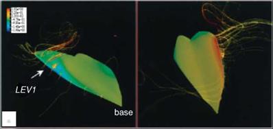
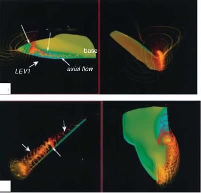
Figure 3.12. Wing surface pressure and streamlines revealing the vortical structures from a 3D numerical simulation of a hovering hawkmoth [247]. (a) Positional angle ф = 30°; (b) ф = 0°; (c) ф = -36°. Reynolds number is approximately 4.0 x 10³ and the reduced frequency is 0.37.
attached throughout the half-stroke without breaking up. Based on these considerable differences between fruit fly and hawkmoth models, Birch and Dickinson [254] hypothesized that the attenuating effect of the downwash induced by the tip vortex and wake vorticity limits the growth of the LEV by lowering the effective AoA and prolonging the attachment of the LEV. Recently, using the time-resolved scanning tomography PIV technique David et al. [282] reported that, in the case of a translating
NACA 0012 wing with the AoA of 45° at Re of 1.0 x 10³, the tip downwash that originates from the formation of TiV indeed reduces the effective AoA and hence also the spanwise vorticity production at the leading edge. However, it should be noted that a NACA 0012 wing is relatively thicker than the model hawkmoth and fruit fly wing.
Another study [256] on large red admiral butterflies, Vanessa Atlanta, questioned the existence of axial flow even at the level of the Reynolds numbers comparable to that of hawkmoths. Using smoke trails to visualize the wake behind free-flying butterflies in a wind tunnel, the investigators showed that the LEV spreads from the wing surface to the body of the animal. In contrast to the conical LEV observed in the hawkmoth, the butterfly LEV exhibits a more cylindrical-shaped vortex with constant diameter, and at the end it connects with the tip vortex. Because the helical structure of the LEV is much weaker on a butterfly wing, the general role of axial flow for stabilizing the LEV was again questioned.
Thomas et al. [258] showed that dragonflies attain lift by generating high-lift LEVs using free – and tethered-flight flow visualization. Specifically, in normal free flight, dragonflies use counter stroke kinematics with an LEV on the forewing down- stroke and with attached flow on the forewing upstroke and on the hindwing throughout. When the dragonflies accelerate, they switch their kinematics to in-phase wing beats with highly separated downstroke flows, with a single LEV attached across both the fore – and hindwings. Based on their flow visualizations, Thomas and coworkers also suggested that the spanwise flow is not a dominant feature of the flow field. They observed that the spanwise flow sometimes runs from the wingtip only to the centerline, or vice versa, depending on the degree of sideslip. The LEV formation always coincided with the rapid increases in AoA. Furthermore, they reckoned that the flow fields produced by dragonflies differ qualitatively from those published for mechanical models of dragonflies, fruit flies, and hawkmoths, which preclude natural wing interactions. However, parametric assessment showed that, provided the Strouhal number is appropriate and the natural interaction between left and right wings can occur, even a simple plunging plate can reproduce the detailed features of the flow seen in dragonflies. Thomas et al. [258] suggested that stability of the LEV is achieved by a general mechanism whereby the flapping kinematics is configured such that an LEV would be expected to form naturally over the wing and remain attached for the duration of the stroke.
Birch et al. [283] conducted flow visualization around a robotic fruit fly model wing and also noticed that, although the LEV remains stable at both lower (Rep = 1.2 x 10²) and higher (Rep = 1.4 x 10³) Reynolds numbers, the flow changes from a relatively simple pattern at lower Reynolds numbers to spiral flow at higher Reynolds numbers. Vorticity measurements taken at mid-stroke, in a plane located at 0.65 of the wing length and perpendicular to the spanwise direction, show stronger and larger LEVs for the higher Reynolds numbers associated with intense axial (spanwise) velocity within the LEV core, with magnitudes significantly larger than those of the tip velocity [254]. At a lower Reynolds number, they observed no peak in axial flow in the area of the LEV core, likely because of the stronger viscous effect.
Kim and Gharib [284] experimentally studied spanwise flow generated by a flat plate by rotating and translating motions with a constant AoA of 45° at a Re of 1.1 x 10³. They observed that, for the translating plate, an LEV develops nonuniformly along the span because of the influence of the wingtip. This deformed LEV induces the spanwise flow over the flat plate and subsequent vorticity transport. However, the spanwise flow is not strong enough to suppress the growth of the LEV near the central region of the plate. For the rotation mode, the vorticity of the LEV is tilted because the size of the LEV increases from the base to the tip. The tilted vorticity induces the spanwise flow over the rotating plate. Contrary to the translation mode, the spanwise flow is also found in the wake; this spanwise flow is due to the streamwise component of vorticity, which is distributed inside a shear layer and a starting vortex in the wake.
The LEV of a flapping wing resembles that of a fixed delta wing. The delta wing owes much of the lift that it is able to generate to the fact that the vortex flow initiates at the leading edge of the wing and rolls into a large vortex over the leeward side, containing a substantial axial velocity component. This high-flow velocity in the core of the vortex is a region of low pressure that generates a suction (i. e., lift). For a delta wing placed at high AoAs, vortex breakdown occurs, causing the destruction of the tight and coherent vortex. The diameter of the core increases, and the axial velocity component is no longer unidirectional. With the loss of axial velocity the pressure increases, and consequently, the wing loses lift. The literature on the subject is immense, and for a more general presentation of the various aspects of vortex breakdown, we refer the reader to several review articles [164] [285] [286]. For a fixed wing, an important trend is that, at a fixed AoA, if the swirl is strengthened, then vortex breakdown occurs at lower Reynolds numbers. In contrast, a weaker swirling flow tends to break down at a higher Reynolds number. Since the fruit fly exhibits a weaker LEV, from this viewpoint, it tends to better maintain the vortex structure than a hawkmoth, which creates a stronger LEV.
Of course, the link between the vortex breakdown and a fixed or flapping wing, if any, is not established. It should be noted that, although helicopter blade models have been used to help explain flapping-wing aerodynamics, spanwise axial flows are generally thought to play a minor role in influencing helicopter aerodynamics [287]. In particular, helicopter blades operate at substantially higher Reynolds numbers and lower AoA. The much higher AR of a blade also makes the LEV harder to anchor.
As previously discussed with geometric and kinematic similarities, the dynamic similarity can be maintained by scaling up the wing dimension while appropriately lowering the flapping frequency, thereby rendering the Reynolds number and the reduced frequency unchanged. For example, Ellington et al. [199] used a robotic wing model to investigate flow over the wings of a hovering hawkmoth and discovered that the LEV spiraled out toward the wingtip. Their findings provided a qualitative explanation of one particular high-lift mechanism. Dickinson et al. [201] also used a robotic wing model representing a fruit fly to directly measure the forces and visualize the flow patterns around the flapping wing. They demonstrated two force peaks during the rotation phase: (i) the rotational mechanism associated with fast pitch-up and (ii) the wake-capture mechanism resulting from the airfoil and wake interactions. Although different explanations of the two force-generation mechanisms have been offered, as described in the following section, it is clear that a robotic model provides an insightful experimental framework in studying flapping wing flight. Furthermore, Birch and Dickinson [254] observed substantially different
|
Table 3.1. Morphological and flight parameters for selected species
|
flow patterns around the same model used in their previous work [201] at different Reynolds numbers (moths and flies) and investigated the impact of the scaling parameters on the aerodynamic outcome. Further refining the experimental techniques, Fry et al. [228] recorded the wing and body kinematics of free-flying fruit flies performing rapid flight maneuvers with a 3D infrared high-speed video and “replayed” them on their robotic model to measure the aerodynamic forces produced by the wings. They reported that the fruit fly generates sufficient torque for rapid turn with subtle modifications in wing motion and suggested that inertia, not viscous force, dominates the flight dynamics of flies. In addition, numerous studies using flow visualization around biological flyers have been conducted, including smoke visualizations [255]-[260] and particle image velocimetry (PIV) measurements [14] [30] [260]-[269] to understand their flight mechanisms. Furthermore, the advance of such experimental technologies has enabled researchers to obtain not only 2D but also 3D flow structures around biological flyers [262] [266]-[269] and/or scaled models [270]-[272] with reasonable resolution in space. For example, Srygley and Thomas
[256] reported a study on the force-generation mechanisms of free-flying butterflies using high-speed, smoke-wire flow visualizations to obtain qualitative images of the airflow around flapping wings. They observed clear evidences of LEV structures. In comparison, in moth and fly flight, the helical structure and the spanwise, axial flow patterns appear to be much weaker. They suggested that free-flying butterflies use a variety of aerodynamic mechanisms to generate force, such as wake capture, LEVs, active and inactive upstrokes, rapid rotation, and clap-and-fling mechanisms. These different mechanisms, discussed in subsequent sections, are often used in successive strokes as seen during takeoff, maneuvering, maintaining steady flight, and landing.
Warrick et al. [14] used PIV to observe the wake around hovering hummingbirds (see Fig. 1.11). They estimated the aerodynamic force based on the circulation computed by integrating the measured vorticity field and observed an asymmetry in the force between upstroke and downstroke. Specifically, hummingbirds generate 75 percent of the lift during the downstroke and 25 percent during the upstroke. They reported an inversion of the cambered wings during the upstroke, as well as evidence of the formation of LEVs, created during the downstroke. Videler et al. [30] measured the flow around a single swift wing in fast gliding in a water-tunnel experiment using the digital particle image velocimetry (DPIV) technique. Their results show that the gliding swifts can generate stable LEVs at small AoAs (5°- 10°). Whereas the swept-back hand wings generate lift using the LEVs, the flow around the arm wings seems to remain attached.
This discussion presents a sample of experimental and modeling investigations. Clearly, depending on the size and flow parameters of individual species, various lift – enhancement mechanisms are observed. In the following discussion, we address the flapping wing aerodynamics by focusing on the unsteady flow mechanisms, as well as related scaling, geometric, and kinematic parameters. Overall, several unsteady aerodynamic mechanisms associated with flapping wing aerodynamics for force generation have been reported in the literature:
(i) delayed stall of LEVs
(ii) lift peak due to pitch-up rotation
(iii) wake capture due to vortical flow and airfoil interactions
(iv) tip vortex
(v) a persistent downward jet in the wake region
(vi) clap-and-fling mechanism
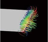
Figure 3.10 displays these mechanisms. In the upper left corner, the wake-capture mechanism, which occurs near the beginning of the translation, is illustrated. This mechanism produces an increase in aerodynamic lift by transferring fluid momentum associated with large-scale vortical flow shed from the previous stroke to the wing at the beginning of each half-stroke. The LEV and its delayed stall are shown in the upper right corner, whereas in the lower right corner, the downward jet is depicted in the wake of a hovering wing. The delayed-stall phenomenon has been investigated from both the dynamic-stall [201] [273] and upper-wing LEV [43] [199] viewpoints. Finally, the tip vortices are shown in the lower left corner via the instantaneous streamlines colored by their vertical velocity components. The impact
 |
|
 |
|
Z-vorticity contours ^
Vertical velocity contours on streamlines
Figure 3.10. Illustration of the time-dependent flow structures affecting the aerodynamics of flapping airfoil during the stroke cycle. Upper left: starting vortices and wake capture. Lower left: tip vortices. Upper right: delayed stall and leading edge vortex. Lower right: jet interaction.
of these mechanisms on the lift and thrust associated with a flapping wing is discussed later.
The Strouhal number (St) is well known for characterizing the vortex dynamics and shedding behavior for flows around a stationary cylindrical object, such as the von Karman vortex street behind a cylindrical object, and for characterizing induced unsteady flows about 2D airfoils undergoing pitching and plunging motions. At certain Strouhal numbers, the pitching and plunging airfoils produce forward thrust,
and the vortices in the wake have a flow structure that is similar to the von Karman vortex street, but with reversed direction of vorticity. Such vortex structures are named reverse von Karman vortices [179]. In general, for flapping flight, the dimensionless parameter St describes the dynamic similarity between the wing velocity and the characteristic velocity; it is usually defined as
St — fLref — 2 fha (3_9)
St ■ ^ref ■ U ■ (39)
This definition offers a measure of propulsive efficiency in flying and swimming animals. For natural flyers and swimmers in cruising conditions, it was found that the Strouhal number is within a narrow region of 0.2 < St < 0.4 [186] [ 249]. For hovering motions, the Strouhal number has no specific meaning because the reference velocity is also based on the flapping velocity.
In addition to the Strouhal number, an important dimensionless parameter that characterizes the unsteady aerodynamics of pitching and plunging airfoils is the reduced frequency, defined in Eq. (1-19). In hovering flight, for which there is no forward speed, the reference speed Uref is defined as the mean wingtip velocity 2Ф fR, and the reduced frequency can be reformed as
![]() k _ 2n fLref n
k _ 2n fLref n
= 2Uref = ФAR ^
where the aspect ratio AR is introduced here again as in Eq. (1-7). For the special case of 2D hovering airfoils, here the reference velocity Uref is the maximum translational flapping velocity, and the reduced frequency is defined as
![]() k 2n fLref cm
k 2n fLref cm
2Uref 2ha
which is the inverse of the normalized stroke amplitude. Based on the definition of the reference velocity and reduced frequency, the airfoil kinematics Eqs. (3-4) and (3-5) can be rewritten as
![]()
![]() h(t jT) = ha sin(2kt/T + у)
h(t jT) = ha sin(2kt/T + у)
a(t/T) = a0 + aa sin(2kt/T)
where t/Tis a dimensionless time, which is non-dimensionalized by a reference time T. Another interpretation of the reduced frequency is that it gives the ratio between the fluid convection time scale, T, and the motion time scale, 1/f.
In the case of forward flight, another dimensionless parameter is the advance ratio, J. In a 2D framework, J is defined as
which is related to St because J = 1 /(nSt). In Eq. (3-14), the reference velocity (Uref) is the forward flight velocity (U).
With the reduced frequency the 3D wing kinematics as illustrated in Eqs. (3-1), (3-2), and (3-3) can be further reformed as
3
ф(/T) = [фт cos(2nkt/T) + фт sin(2nkt/T)], (3-15)
3
в (t/T) = [6cn cos(2nkt/T) + esn sin(2nkt/T)], (3-16)
3
a(t/T) = [acn cos(2nkt/T) + asn sin(2nkt/T)], (3-17)
where t/T is a dimensionless time, which is non-dimensionalized by a reference time T, resulting in a dimensionless period of п /k.
If we choose cm, Uref, and 1 /f as the length, velocity, and time scales, respectively, for non-dimensionalization, then the corresponding momentum equation for constant density fluid yields
![]() (3-18)
(3-18)
where * designates a dimensionless variable. The reduced frequency and Reynolds number appear in the momentum equation, whereas the Strouhal number comes up in the kinematics.
Morphological and flight parameters for the fruit fly (Drosophila melanogaster), bumblebee (Bombus terrestris), hawkmoth (Manduca sexta), and hummingbird (Lampornis clemenciae) are summarized in Table 3.1. For all these flyers, the flapping frequency is around 20-200 Hz, and the flight speed is about several m/s, yielding a Reynolds number from 102 to 104 based on the mean chord and the forward flight speed. In this flight regime, the unsteady, inertia, pressure, and viscous forces are all important.
The aerodynamics of biological flight can be modeled in the framework of unsteady, Navier-Stokes equations around a body and two or four wings. Nonlinear physics with multiple variables (velocity and pressure) and time-varying geometries are among the aspects of primary interest.
Scaling laws are useful to reduce the number of parameters, to clearly identify the physical flow regimes, and to offer guidelines to establish suitable models for predicting the aerodynamics of biological flight. Three main dimensionless parameters in the flapping flight scaling are (i) the Reynolds number (Re), which represents the ratio of inertial and viscous forces; (ii) the Strouhal number (St), which describes the relative influence of forward versus flapping speeds in forward flight; and (iii) the reduced frequency (k). The reduced frequency measures unsteadiness by comparing the spatial wavelength of the flow disturbance to the chord [186]. Together with geometric and kinematic similarities, the Reynolds number, the Strouhal number, and the reduced frequency are sufficient to define the aerodynamic similarity for a rigid wing.
3.2.1 Reynolds Number
The Reynolds number represents the ratio between inertial and viscous forces. Given a reference length Lref and a reference velocity Uref, one defines the Reynolds number Re as
U fL f
Re = ref ref j (3-6)
V
where v is kinematic viscosity of the fluid. In flapping wing flight, considering that flapping wings produce the lift and thrust, either a mean chord length cm or a wing length R is commonly used as the reference length, whereas the body length is typically used in swimming animals. Note that the definition of mean chord length is an averaged chord length in the spanwise direction. The reference velocity Uref is the
free-stream velocity in forward flight, but it is defined differently in hovering flight. In hovering, the mean wingtip velocity may be used as the reference velocity, which is also written as Uref = 2Ф fR, where Ф is the wing-beat amplitude (measured in radians). Therefore, the Reynolds number for a 3D flapping wing, Ree, in hovering flights can be cast as
. UrefLref 2Ф fRcm 2Ф fR2 4_
f3 V V V AR
where the aspect ratio AR as described in Chapter 1 has been introduced in a form of AR = 4R2/S, with the wing area being the product of the wingspan (2R) and cm. Note that the Reynolds number here is proportional to the wing-beat amplitude, the flapping frequency, and the square of the wing length, R2, but is inversely proportional to the AR of the wing. In insect flights, the wing-beat amplitude and the aspect ratio of the wing do not vary significantly, whereas the flapping frequency increases as the insect size is reduced. In general these characteristics result in Re ranging from ^(Ю1) to 0(104). In addition, given a geometrically similar wing model that undergoes flapping hovering with the same wing-beat amplitude, the product of fR2 can preserve the same Reynolds number. This implies that a scaled-up but low- flapping-frequency wing model can be built mechanically to mimic insect flapping flight based on the aerodynamic similarity. In fact, robotic model-based studies [199] [201] have been established on such a basis provided that the second parameter, the reduced frequency, can be satisfied simultaneously.
The Reynolds number can also be defined with an alternative reference length and/or reference velocity. For example, using the wing length R as the reference length and the wing velocity, Uref = 2n fr2R, where r2 is the radius of the second moment of wing area (approximately 0.52 for the hawkmoth, Manduca sexta [247] [248]), the Reynolds number Re^ is proportional with (ФfR2)/v and is not dependent on the aspect ratio of the wing. Note that the reference velocity here is almost half of that at the wingtip.
For a 2D hovering wing, the Reynolds number can be defined by the maximum plunging velocity given by Eq. (3-8a) or by the mean plunging velocity, Eq. (3-8b), with a factor of n/2 difference. Both definitions have their benefits, but in this chapter, we use Eq. (3-8b) as the Reynolds number for a 2D hovering motion unless stated otherwise.
UrefLref 2n fhacm
Re f 2 = V = V ’ (3-8a)
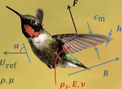
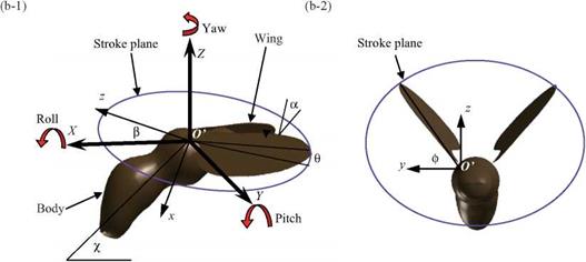
Figure 3.5 illustrates the wing and body movement of a hummingbird, as well as definitions of some key terms used in this section. The body kinematics is represented by the body angle x (inclination of the body), which is relative to the horizontal plane, and by the stroke plane angle в (indicated by the solid lines), which is defined
(a)
|
|
|
Figure 3.5. (a) Physical variables shown in the case of a hummingbird, (b) Schematic diagram of coordinate systems and wing kinematics, (b-1) The local wing-base-fixed and the global space-fixed coordinate systems. The local wing-base-fixed coordinate system (x, y, z) is fixed on the center of the stroke plane (origin O’ at the wing base) with the д-direction normal to the stroke plane, the у-direction vertical to the body axis, and the z-direction parallel to the stroke plane; (b-2) definition of the positional angle ф, the feathering angle (AoA) a, and elevation angle ф of the flapping wing, the body angle y, and the stroke plane angle ft. |
as the plane that includes the wing base and the wingtip’s positions at the maximum and the minimum sweep. The wing-beat kinematics is described by three angles relative to the stroke plane: (i) flapping about the л-axis in the wing-fixed coordinate system described by the positional (flapping) angle ф, (ii) rotation of the wing about
the z-axis described by the elevation (deviation) angle в; and (iii) rotation (feathering) of the wing about the у-axis described by the AoA (feathering angle) a. The time history of AoA includes high-frequency modes that are characteristic of some insects [224]. The body angle and the stroke plane angle vary in accordance with the flight speed and flapping wing kinematics of biological flyers [70] [225]. For a general 3D case, a definition of the positional angle, the elevation angle, and the AoA/feathering, all in radians, can be given as follows, for the first four modes:
3
ф() = 0 [Фсп cos (2nn ft) + fsn sin (2nn ft)], (3-1)
n=0
3
в (t) = [ecn cos (2nn ft) + esn sin (2nn ft)], (3-2)
3
a (t) = [acn cos (2nn ft) + asn sin (2nn ft)], (3-3)
Note that n indicates the order of the Fourier series. The Fourier coefficients Фсп, фт, ecn, esn, acn, and asn can be determined from the empirical and measured kinematics data. Wing and body kinematics of biological flyers can be measured by high-speed cameras [226]-[234], laser techniques (a scanning projected line method [235], a reflection beam method [236], a fringe shadow method [237], and a projected comb fringe method [238]), and a combination of high-speed cameras and a projected comb-fringe technique with the Landmarks procedure [239]. Advancement in measurement techniques also enables quantification of flapping wing and body kinematics along with the 3D deformation of the flapping wing. Recently, data on the instantaneous wing kinematics involving camber along the span, twisting, and flapping motion have been reported (e. g., a hovering honeybee [240], a hovering hoverfly [241], a free-flying hawkmoth [242], and a bat [243]). Clearly, these efforts have helped establish more complex and useful computational models as well as to develop bio-inspired MAVs. Examples of the kinematics of a hovering hawkmoth [226] and free-flying hoverflies are plotted in Figure 3.6.
Although 3D effects are important for predicting low Reynolds number flapping wing aerodynamics, 2D experiments and computations do provide valuable insight into the unsteady fluid physics related to flapping wings. Tang, Viieru, and Shyy [244] discussed two hovering modes that are observed in nature: the “water treading” mode [175] and the “normal hovering” mode [217]. The plunging and pitching of the airfoil are described by symmetric, periodic functions:
|
h (t) = ha sin (2n ft + ф), |
(3-4) |
|
a (t) = a0 + aa sin (2n ft), |
(3-5) |
where ha is the plunging amplitude, f is the plunging frequency, a0 is the initial pitching angle, aa is the pitching amplitude, and ф is the phase difference between plunging and pitching motion. The schematics of the two hovering modes are presented in Figure 3.7. The initial pitching angle for the water treading mode is zero (a0 = 0°), whereas for the normal-flapping/hovering mode a0 = 90°. Figure 3.8 shows
 |
other 2D flapping motions – the pitching and plunging motions – that are more commonly observed for forward flight. The fluid dynamics based on these kinematics are highlighted in Section 3.5.
For normal hovering, based on the phase relationship between the translation and rotation of the wing, Dickinson et al. [201] categorized the wing motion into advanced (<p > 90°), synchronized (<p = 90°), and delayed modes (<p < 90°). The
advanced mode (Fig. 3.9a) is the pattern in which the wing rotates before it reverses direction at the end of each stroke. The synchronized mode (Fig. 3.9b) is the pattern
![]()
|
|
|
|
|
|
|
|
|
|
|
|
|
|
|
|
|
|
|
|
|
|
|
|
|
|
|
|
|
|
 |
|
|
|
|
|
|
|
|
|
![]()
![]()
![]()

Figure 3.9. Schematics of the three wing rotation patterns: (a) advanced, (b) synchronized, and (c) delayed rotation. As shown in Dickinson et al. [201], the timing of the wing rotation plays an important role in lift generation and, consequently, in maneuvering.
in which the wing rotation synchronizes with its translational motion: its AoA is 90° at the end of each stroke. The delayed mode (Fig. 3.9c) is the pattern in which the wing rotates after it reverses direction at the end of each stroke. Discussion of the effects of the phase relationship on aerodynamic performance is given in Section 3.4.1.