Category AN INTRODUCTION TO FLAPPING WING AERODYNAMICS

Because of the influence of flow separation and laminar-turbulent transition, the preferred airfoil shapes in the low Reynolds number regime are different from those

Figure 2.10. Streamlines and turbulent shear stress for the AoA = 11°. (a) experimental measurement by Rade – spiel et al. [135] and (b) numerical sim­ulation with N = 8 by Lian and Shyy [117].

in the high Reynolds number regime. Furthermore, in addition to the Reynolds num­ber, the airfoil camber, thickness, surface smoothness, free-stream unsteadiness, and aspect ratio all play important roles in determining the aerodynamic performance of a low Reynolds number flyer. These factors are discussed in this section.

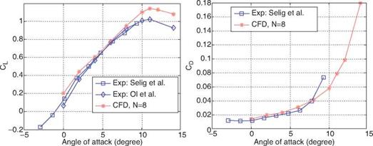
Lian and Shyy [117] studied the Reynolds number effect with a Navier-Stokes equation solver augmented with the eN method. The lift and drag coefficients of the SD7003 airfoil against AoA are plotted in Figure 2.6. This figure vividly shows the good agreement between the numerical results [117] and the experimental measurements by Ol et al. [134] and Selig et al. [88]. Both the simulation and the mea­surement by Ol et al. [134] predict that the maximum lift coefficient happens at the AoA = 11°. Close to the stall AoA, the simulations over-predict the lift coefficients.

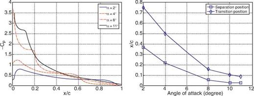
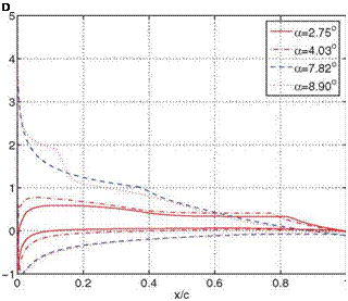
As the AoA increases, as illustrated in Figure 2.7, the adverse pressure gradient downstream of the point of suction peak becomes stronger and the separation point moves toward the leading edge. The strong pressure gradient amplifies the distur­bance in the separation zone and prompts transition. As the turbulence develops, the increased entrainment causes reattachment. At an AoA of 2°, the separation position is at around 37 p of the chord length, and transition occurs at 75 percent of the chord length. A long LSB forms. The plateau of the pressure distribution shown in Figure 2.7a is characteristic of an LSB. As seen in Figure 2.7b the bubble length decreases with an increase in the AoA.

Lian and Shyy [117] compared computed shear stress with experimental mea­surements by Radespiel et al. [135], using the low-turbulence wind tunnel and the

water tunnel because of its low-turbulent nature. Radespiel et al. [135] suggested that large values of critical N factor should be appropriate. As shown in Figure 2.8, the simulation by Lian and Shyy [117] with N = 8 shows good agreement with measurements in terms of the transition position, reattachment position, and vortex core position. It should be noted that, in the experiment, the transition location is defined as the point where the normalized Reynolds shear stress reaches 0.1 percent and demonstrates a clearly visible rise. However, the transition point in the simu­lation is defined as the point where the most unstable TS wave has amplified over a factor of eN. This definitional discrepancy may cause some problems when we compare the transition position. In any event, simulations typically predict notice­ably lower shear-stress magnitude than the experimental measurement. Recently, LES simulations of an SD7003 rectangular wing at the Reynolds number of 6×104 were performed by Galbraith and Visbal [136] and Uranga et al. [137]; they discussed transition mechanisms based on instantaneous and phase-averaged flow features and

Figure 2.8. Streamlines and turbulent shear stress for the AoA = 4°. (a) Experimental measurement by Rade – spiel et al. [135] and (b) numerical sim­ulation with N = 8 by Lian and Shyy

[117].

turbulence statics. Moreover, using time-resolved particle image velocimetry (PIV), Hain et al. [138] studied the transition mechanism in the flow around an SD7003 wing at Reynolds number of 6.6 x 104; they claimed that the TS waves trigger the ampli­fication of the KH waves, which explains why the size of the separation bubble is affected by the magnitude of the TS waves at separation.

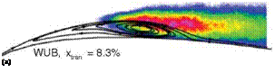
As the AoA increases, both the separation and the transition positions move upstream, and the bubble shrinks. The measurements at the AoAs of 8° and 11° are performed in the water tunnel with a measured free-stream turbulence intensity of 0.8 percent. At the AoA = 8° the simulation by Lian and Shyy [117] predicts that the flow goes though transition at 15 percent of the chord, which is close to the experimental measurement of 14 percent. The bubble covers approximately 8 percent of the airfoil upper surface. The computational and experimental results for the AoA of 8° are shown in Figure 2.9. With the AoA of 11°, the airfoil is close to stall. The separated flow requires a greater pressure recovery in the laminar bubble for reattachment. Lian and Shyy [117] predicted that flow separates at 5 percent of the chord and that the separated flow quickly reattaches after it experiences transition at the 7.5 percent chord position, whereas in the experiment transition actually occurred at 8.3 percent. This quick reattachment generally represents the transition-forcing mechanism. Comparison shows that the computed Reynolds shear stress matches the experimental measurement well (see Fig. 2.10).

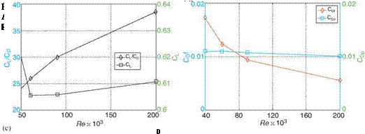
For low Reynolds number airfoils, the chord Reynolds number is a key parame­ter used to characterize the overall aerodynamics. Between the separation position and the transition position, as shown in Figure 2.11a, the shape factor H and the momentum-thickness-based Reynolds number increase with the chord Reynolds number. As shown in Figure 2.11b the effective airfoil shape, which is the superim­position of the airfoil and the boundary-layer displacement thickness, has the largest camber at the Reynolds number Re = 4 x 104. This helps explain why the largest lift coefficient is obtained at that Reynolds number (see Fig. 2.11c). The camber decreases significantly when the Reynolds number increases from 4 x 104 to 6 x 104,

Figure 2.9. Streamlines and turbulent shear stress for the AoA = 8°. (a) Exper­imental measurement by Radespiel et al. [135] and (b) numerical simulation with N = 8 by Lian and Shyy [117].

but does not show considerable change when the Reynolds number increases further. Therefore one does not observe much increase in the lift coefficient even though the LSB length is shorter at higher Reynolds numbers. One can conclude from Figure 2.11d that the enhancement of lift-to-drag ratio is mainly due to the reduction of friction drag at high Reynolds numbers. As the Reynolds number increases, the form drag does not vary as much as does the friction drag.

In this section we offer a more detailed presentation of the eN method, because it forms the basis for low Reynolds number aerodynamics predictions and has proven to be useful for engineering applications. As already mentioned, the eN method is based on linear stability analysis, which states that transition occurs when the most unstable TS wave in the boundary layer has been amplified by a certain factor. Given a velocity profile, one can determine the local disturbance growth rate by solving the Orr-Sommerfeld eigenvalue equations. Then, the amplification factor is calculated by integrating the growth rate, usually the spatial growth rate, starting from the point of neutral stability. The Transition Analysis Program System (TAPS) by Wazzan and co-workers [125] and the COSAL program by Malik [126] can be used to compute the growth rate for a given velocity profile. Schrauf also developed a program called Coast3 [127]. However, it is very time consuming to solve the eigenvalue equations. An alternative approach was proposed by Gleyzes et al. [128], who found that the integrated amplification factor n can be approximated by an empirical formula as follows:

dn

n= (H)[Ree – Ree(H)], (2-12)

dRee o

where Ree is the momentum thickness Reynolds number, Ree is the critical Reynolds number that we define later, and H is the shape factor previously discussed. With this approach, one can approximate the amplification factor with a reasonably good accu­racy without solving the eigenvalue equations. For similar flows, the amplification factor n is determined by the following empirical formula:

dn

= 0.01{[2.4H – 3.7 + 2.5 tanh (1.5H – 4.65)]2 + 0.25}1/2. (2-13)

dR. ee

For non-similar flows (i. e., those that cannot be treated by similarity variables using the Falkner-Skan profile family [129]) the amplification factor with respect to the spatial coordinate f is expressed as

dn = dn 1/ f due Л Pиев21

df dReg 2 ue df uef в

An explicit expression for the integrated amplification factor then becomes

f dn

n (f) = — df, (2-15)

fo df

where f0 is the point where Ree = Ree, and the critical Reynolds number is expressed

eo

by the following empirical formulas:

/1415 / 20 3 295

log10Reeo = [HZTi – 0.489J tanh —— – 12.9 j + H-j + 0.44. (2-16)

Once the integrated growth rate reaches the threshold N, flow becomes turbulent. To incorporate the free-stream turbulence level effect, Mack [130] proposed the following correlation between the free-stream intensity 7) and the threshold N:

N = -8.43 – 2.4 1п(7), 0.0007 < Ti < 0.0298. (2-17)

However, care should be taken in using such a correlation. The free-stream tur­bulence level itself is not sufficient to describe the disturbance, and other information, such as the distribution across the frequency spectrum, should also be considered. The so-called receptivity – how the initial disturbances within the boundary layer are related to the outside disturbances – is a critically important issue. Actually, we can only determine the N factor if we know the “effective 7),” which can be defined only through a comparison of the measured transition position with calculated amplifica­tion ratios [131].

A typical procedure to predict the transition point using coupled RANS equa­tions and the eN method is as follows. First, solve the Navier-Stokes equations together with a turbulence model without invoking the turbulent production terms, for which the flow is essentially laminar; then integrate the amplification factor n based on Eq. (2-12) along the streamwise direction; once the value reaches the threshold N, the production terms are activated for the post-transition computa­tions. After the transition point, flow does not immediately become fully turbulent;

instead, the movement toward full turbulence is a gradual process. This process can be described with an intermittency function, allowing the flow to be represented by a combination of laminar and turbulent structures. With the intermittency function, an effective eddy viscosity is used in the turbulence model and can be expressed as follows:

vTe = Y VT,

where y is the intermittency function and vTe is the effective eddy viscosity.

In the literature a variety of intermittency distribution functions have been pro­posed. For example, Cebeci [132] presented such a function by improving a model previously proposed by Chen and Thyson [133] for the Reynolds number range of 2.4 x 105 to 2 x 106 with an LSB. However, no model is available when the Reynolds number is lower than 105. Lian and Shyy [117] suggested that, for separation-induced transition at such a low Reynolds number regime, the intermittency distribution is largely determined by the distance from the separation point to the transition point: the shorter the distance, the quicker the flow becomes turbulent. In addition, previ­ous work suggested that the flow property at the transition point is also important. From the available experimental data and our simulations, Lian and Shyy [117] proposed the following model:

where xT is the transition onset position, xS is the separation position, HT is the shape factor at the transition point, and ReeT is the Reynolds number based on the momentum thickness at the transition point.

The constant property Navier-Stokes equations adequately model the fluid physics needed to perform practical laminar – and turbulent-flow computations in the Reynolds number range typically used by the low Reynolds number flyers:

^ = 0,

д X:

д U: d 1 d p d2

—- + —— (U:U j ) =——– + V (U: ),

dt d Xj 1 p d X : дX2-

where u: are the mean flow velocities and v is the kinematic viscosity. For turbulent flows, turbulent closures are needed if one is solving the ensemble-averaged form of the Navier-Stokes equations. Numerous closure models have been proposed in the literature [102]. Here we present the two-equation к — ю turbulence model [102] as an example. For clarity, the turbulence model is written in Cartesian coordinates as follows:

For the preceding equations, k is the turbulent kinetic energy, m is the dissipation rate, vT is the turbulent kinematic eddy viscosity, ReT is the turbulent Reynolds number, and а0, в, R^, Rk, and Rm are model constants. To solve for the transition from laminar to turbulent flow, the incompressible Navier-Stokes equations are coupled with a transition model.

The onset of laminar-turbulent transition is sensitive to a wide variety of disturbances, as produced by the pressure gradient, wall roughness, free-stream turbulence, acoustic noise, and thermal environment. A comprehensive transition model considering all these factors currently does not exist. Even if we limit our focus to free-stream turbulence, it is still a challenge to provide an accurate mathe­matical description. Overall, approaches to transition prediction can be categorized as (i) empirical methods and those based on linear stability analysis, such as the eN method [96]; (ii) linear or non-linear parabolized stability equations [103]; and (iii) large-eddy simulation (LES) [104] or direct numerical simulation (DNS) methods [105].

Empirical methods have also been proposed to predict transition in a sepa­ration bubble. For example, Roberts [93] and Volino and Bohl [106] developed models based on local turbulence levels; Mayle [107], Praisner and Clark [108], and Roberts and Yaras [109] tested concepts by using the local Reynolds num­ber based on the momentum thickness. These models use only one or two local parameters to predict the transition points and hence often oversimplify the down­stream factors such as the pressure gradient, surface geometry, and surface rough­ness. For attached flow Wazzan et al. [110] proposed a model based on the shape factor H. Their model gives a unified correlation between the transition point and Reynolds number for a variety of problems. For separated flow, however, no similar models exist, in part because of the difficulty in estimating the shape factor.

Among the approaches employing linear stability analysis, the eN method has been widely adopted [111] [112]. It solves the Orr-Sommerfeld equation to evaluate the local growth rate of unstable waves based on velocity and temperature profiles over a solid surface. Its successful application is exemplified in the popularity of airfoil analysis software such as XFOIL [96]. XFOIL uses the steady Euler equa­tions to represent the inviscid flows, a two-equation integral formulation based on dissipation closure to represent boundary layers and wakes, and the eN method to
tackle transition. Coupling the Reynolds-averaged Navier-Stokes (RANS) solver with the eN method to predict transition has been practiced by Radespiel et al. [113], Stock and Haase [114], and He et al. [115]. An application of this approach for low Reynolds number applications can be found in the work of Yuan et al. [116] and Lian and Shyy [117].

The eN method is based on the following assumptions: (i) the velocity and temperature profiles are essentially 2D and steady, (ii) the initial disturbance is infinitesimal, and (iii) the boundary layer is thin. Even though in practice the eN method has been extended to study 3D flow, strictly speaking, such flows do not meet the preceding conditions. Furthermore, even in 2D flow, not all these assumptions can be satisfied [118]. Nevertheless, the eN method remains a practical and useful approach for engineering applications.

Advancements in turbulence modeling have made possible alternative approaches for transition prediction. For example, Wilcox devised a low Reynolds number к – ю turbulence model to predict transition [119]. One of his objectives is to match the minimum critical Reynolds number beyond which the TS wave begins forming in the Blasius boundary-layer context. However, this model fails if the separation-induced transition occurs before the minimum Reynolds number is reached, as frequently occurs in the separation-induced transition. Holloway et al. [120] used unsteady RANS equations to study the flow separation over a blunt body for the Reynolds number range of 104 to 107. It has been observed that the predicted transition point can be too early even for a flat-plate flow case, as illustrated by Dick and Steelant [121]. In addition, Dick and Steelant [122] and Suzen and Huang [123] incorporated the concept of an intermittency factor to model transitional flows. One can model this either by using conditional-averaged Navier-Stokes equations or by multiplying the eddy viscosity by the intermittency factor. In either approach, the intermittency factor is solved based on a transport equation, aided by empirical cor­relations. Mary and Sagaut [124] studied the near-stall phenomena around an airfoil using LES, and Yuan et al. [116] studied transition over a low Reynolds number airfoil using LES.

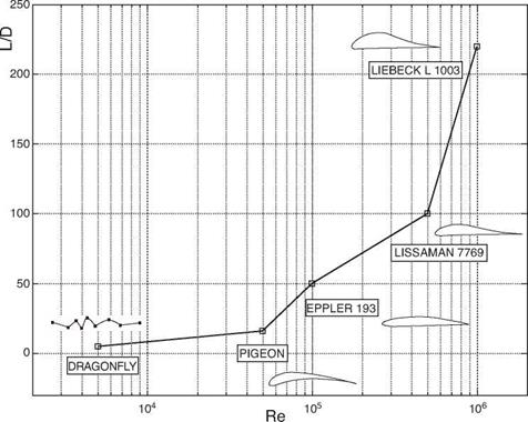
Figure 2.2 illustrates the aerodynamic performance and shapes of several represen­tative airfoils under steady-state free-stream. A substantial reduction in lift-to-drag ratio is observed as the Reynolds number becomes lower. The observed aerody­namic characteristics are associated with the laminar-turbulent transition process. With conventional manned aircraft wings whose Reynolds numbers exceed 106, the flows surrounding them are typically turbulent, with the near-wall fluid capable of strengthening its momentum via energetic “mixing” with the free-stream. Conse­quently, flow separation is not encountered until the AoA becomes high. With low Reynolds number aerodynamics, the flow is initially laminar and is prone to sepa­rate even under a mild adverse pressure gradient. Under certain circumstances, as discussed next, the separated flow reattaches and forms a laminar separation bubble (LSB) while transitioning from a laminar to a turbulent state. Laminar separation can modify the effective shape of an airfoil, and so it consequently influences the aerodynamic performance.

The first documented experimental observation of an LSB was reported by Jones [92]. In general, under an adverse pressure gradient of sufficient magnitude, the laminar fluid flow tends to separate before becoming turbulent. After separation, the flow structure becomes increasingly irregular, and beyond a certain threshold, it undergoes a transition from laminar to turbulent. The turbulent mixing process brings high-momentum fluid from the free-stream to the near-wall region, which can overcome the adverse pressure gradient, causing the flow to reattach.

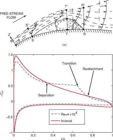
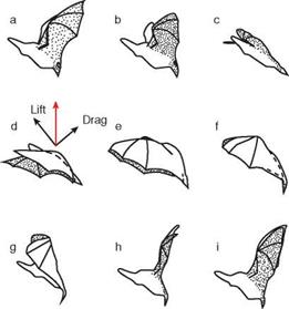
The main features of an LSB are illustrated in Figure 2.3a. After separation, the laminar flow forms a free-shear layer, which is contained between outer edge S”T” of the viscous region and the mean dividing streamline ST’. Downstream of the transition point T, turbulence can entrain a significant amount of high-momentum fluid through diffusion [93], which enables the separated flow to reattach to the wall and form a turbulent free-shear layer. The turbulent free-shear layer is contained between lines T”R” and T’R. The recirculation zone is bounded by the ST’R and STR.

Just downstream of the separation point, there is a “dead-fluid” region, where the recirculation velocity is significantly lower than the free-stream velocity and the flow can be considered almost stationary. Because the free-shear layer is laminar and is less effective in mixing than in turbulent flow, the flow velocity between the separation and transition is virtually constant [93]. That the velocity is almost

constant is also reflected in the pressure distribution in Figure 2.3b. The pressure “plateau” is a typical feature of the laminar part of the separated flow.

The dynamics of an LSB depends on the Reynolds number, pressure distribution, geometry, surface roughness, and free-stream turbulence. An empirical rule given by Carmichael [94] says that the Reynolds number, based on the free-stream velocity and the distance from the separation point to the reattachment point, is approxi­mately 5 x 104. It suggests that, if the Reynolds number is less than 5 x 104, an airfoil will experience separation without reattachment; in contrast, if the Reynolds number is slightly higher than 5 x 104, a long separation bubble will occur. This rule provides general guidance to predict the reattachment, but should be used with caution. As we discuss later, the transition and the reattachment process are too complicated to be described by the Reynolds number alone.

As the Reynolds number decreases, the viscous damping effect increases, and it tends to suppress the transition process or to delay reattachment. The flow will not reattach if the Reynolds number is sufficiently low to enable the flow to com­pletely remain laminar or the pressure gradient is too strong for the flow to reattach.

Thus, without reattachment, a bubble does not form and the flow is then fully separated.

Based on its effect on pressure and velocity distribution, the LSB can be classified as either a short or long bubble [95]. A short bubble covers a small portion of the airfoil and plays an insignificant rule in modifying the velocity and pressure distributions over an airfoil. In this case, the pressure distribution closely follows its corresponding inviscid distribution except near the bubble location, where there is a slight deviation from the inviscid distribution. In contrast, a long bubble covers a considerable portion of the airfoil and significantly modifies the inviscid pressure distribution and velocity peak. The presence of a long bubble leads to decreased lift and increased drag.

Typically, a separation bubble has very steep gradients in the edge velocity, ue, and momentum thickness, в, at the reattachment point, resulting in jumps in Aue and Ав over a short distance. For incompressible flow, the momentum thickness is defined as

в=1′ U (1 – U И <2-d

where u is the streamwise velocity and U is the free-stream velocity. For flow over a flat plate the momentum thickness is equal to the drag force divided by pU[4]. If the skin friction is omitted, the correlation between these jumps can be expressed as

where H is the shape factor, defined as the ratio between the boundary-layer displace­ment thickness S* and the momentum thickness в. The boundary-layer displacement is defined as

delays the transition and elongates the free-shear layer. At this Reynolds number, the separated flow no longer reattaches to the airfoil surface, and the main structures are no longer sensitive to the exact value of the Reynolds number.

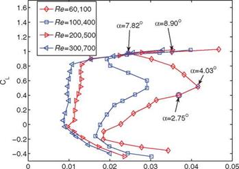
For a fixed Reynolds number, varying the AoA changes the pressure gradient aft of the suction peak and therefore changes the LSB. In this aspect, varying the AoA has the same effect on the LSB as changing the Reynolds number. Figure 2.5 illustrates that, at a fixed Reynolds number of 6.01 x 104for the Eppler E374, a zigzag pattern appears in the lift-drag polar: [5] 2

(c)

3. When the AoA is further increased (beyond 7.82°), the separated flow quickly experiences transition; however, with a massive separation, the turbulent diffu­sion can no longer make the flow reattach, and the drag increases substantially with little changes in lift.

The previously described zigzag pattern of the lift-drag polar is a noticeable feature of low Reynolds number aerodynamics. As illustrated in Figure 2.5, at a sufficiently high Reynolds number, the polar exhibits the familiar C-shape.

Earlier experimental investigations on low Reynolds number aerodynamics were reviewed by Young and Horton [97]. Carmichael [94] further reviewed the­oretical and experimental results of various airfoils with Reynolds numbers span­ning from 102 to 109. In particular, many investigators studied the near-surface flow and aerodynamic loads of a wing at Reynolds numbers in the range of 104 to 106. Crabtree [98] studied the formation of short and long LSBs on thin air­foils. Consistent with the preceding discussion of the two types of separation bub­bles, he suggested that the long bubble directly influences aerodynamic character­istics, whereas the short one serves as an agent for initiating a turbulent boundary layer.

In the last two decades, numerous investigations have been reported on the interplay between the near-wall flow structures and aerodynamic performance. For example, Huang et al. [99] studied the aerodynamic performance versus the surface – flow mode at different Reynolds numbers. Hillier and Cherry [100] and Kiya and Sasaki [101] studied the influence of the free-stream turbulence on the separation bubble along the side of a blunt plate with right-angled corners, finding that the bubble length, sizes of vortices in the separating region, and level of the suction peak pressure can all be well correlated with the turbulence outside the shear layer and near the separation point.

In this chapter, we have offered an overview of the various low Reynolds number flyers, discussing simple mechanics for several flight modes and highlighting flight characteristics and scaling laws related to wingspan, wing area, wing loading, wing – beat frequency, and vehicle size and weight.

The scaling laws indicate that, as a flyer’s size reduces, it has to flap faster to stay in the air, experiences lower wing loading, is capable of cruising slower, has a lower stall speed, and, consequently, can survive much better in a crash landing. In addition, as a flyer becomes smaller, its weight shrinks at a much faster rate, meaning that it can carry very little “fuel” and has to resupply frequently. Birds, bats, and insects apply different flapping patterns in hovering and forward flight to generate lift and thrust. Typically, in slow forward flight the reduced frequency and wing-beat amplitude tend to be high, resulting in highly unsteady flow structures. In fast forward flight the reduced frequency and the wing-beat amplitude tend to be low, and the wake often consists of a pair of continuous undulating vortex tubes or line vortices. Larger birds have relatively simple wingtip paths in comparison to smaller flyers. We have also discussed the power requirement associated with flight, including the L-shaped curve between specific power and flight speed.

As a flyer’s size reduces, its operating Reynolds number becomes lower. As detailed later, the lift-to-drag ratio of a stationary wing deteriorates as the Reynolds number decreases. Due to the low weight and slower flight speed, a small flyer is substantially more influenced than large flyers by the flight environment such as wind gust. To overcome these challenges, natural flyers improve flight performance, including force generation and maneuverability, using flapping wings and wing-tail coordination. In particular, the fixed-wing design (other than the noticeable exam­ples such as the delta wing) tends to favor flow patterns with no large scale vortical flows, whereas flapping wing flyers, especially smaller species such as humming­birds and insects, generate coherent, large-scale vortical flows with low-pressure

regions. As discussed in detail in Chapter 3, several fluid flow mechanisms, including a leading-edge vortex caused by varying the AoA under dynamic pitch (induced either actively, by arm and muscle, or passively, by structural shape deformation) and spanwise flows associated with modest aspect ratios, among others, contribute to generating necessary lift and thrust. Of course, the movement of the wing, the substantial impact of wind gust and environmental uncertainty, and the associated structural deformation of the wing during flapping make flapping wing aerodynamics more complex and challenging to analyze.

In the next chapter, we summarize the rigid fixed-wing aerodynamics that shares fundamental aspects of low Reynolds aerodynamics such as flow separation, laminar- to-turbulent transition, and so on. In Chapter 3, we discuss rigid flapping wing aero­dynamics and focus on the wing kinematics and the resulting unsteady flow features involving flapping wings. In Chapter 4, we discuss aeroelasticity of flexible flapping wings including both active and passive mechanisms and implications.

As already mentioned, there are several prominent features of MAV flight: (i) low Reynolds numbers (104 to 105), resulting in degraded aerodynamic performance; (ii) small physical dimensions, resulting in much reduced payload capabilities and some favorable scaling characteristics including structural strength, reduced stall speed, and impact tolerance; and (iii) low flight speed, resulting in an order one effect of the flight environment such as wind gust, as well as intrinsically unsteady flight characteristics. The preferred low Reynolds number airfoil shapes are different in thickness, camber, and aspect ratio from those typically employed for manned air­craft. In this chapter, we discuss the low Reynolds number aerodynamics associated with rigid fixed wings, including the implications of airfoil shapes, laminar-turbulent transition, and unsteady free-stream on the performance outcome.

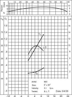
Schmitz [84] was among the first to investigate the aerodynamics for model airplanes in Germany, and he published his research in 1942. His work is often con­sidered to be the first reported low-speed wind-tunnel research. However, experi­mental investigations of low Reynolds number aerodynamics were conducted earlier by Brown [85] and by Weiss [86], in the two (and only) issues of The Journal of Inter­national Aeromodeling. Brown’s experiments focused on curved-plate airfoils, made by using two circular arcs meeting at a maximum camber point of 8 percent, but at varying locations. The wings’ test sections were all 12.7 cm x 76.2 cm, giving an AR of 6. In all cases, the tests were conducted at a free-stream velocity of 94 cm/s. The Reynolds number, although not mentioned in Brown’s study [85], is estimated to be about 8 x 103.

It is hard to judge the quality of the measurements reported in these early works (see Fig. 2.1). Nevertheless, these publications have clearly demonstrated that work with model airplanes offers much to scientific investigation and continues to generate enthusiastic inquiries about many aspects related to low Reynolds number aerodynamics. Representative figures from Brown’s experiments [85] are included here for us to gain a historical perspective.

Many published papers have improved our understanding and experimental database and have provided airfoil design guidance in the lower Reynolds number regime. For example, valuable insight has been offered by Liebeck [87], Selig et al. [88]-[90], and Hsiao et al. [91]. Liebeck [87] has addressed the laminar separation and airfoil design issues for the Reynolds number between 2 x 105 and 2 x 106, and

Hsiao et al. [91] have investigated the aerodynamic and flow structure of an airfoil, NACA 633-018, for the Reynolds number between 3 x 105 and 7.74 x 105. Selig et al. have reported on a wide variety of airfoils with basic aerodynamic data for the Reynolds number between 6 x 104 and 3 x 105 [88] [ 90] and for the Reynolds number between 4 x 104 and 3 x 105 [89]. In the following sections, we discuss the various aerodynamics characteristics and fluid physics for the Reynolds number between 102 and 106, with a focus on issues related to the Reynolds number of 105 or lower.

Like an aircraft, a natural flyer has to generate power to produce lift and to overcome drag during the flight. When soaring or gliding without flapping, the flyer produces much of the power required by converting potential energy to kinetic energy, and vice versa. When the flyer flaps, the power is the rate at which work is produced by the flight muscles. For basic aerodynamic concepts discussed in this section, please refer to the standard textbooks such as Anderson [44] and Shevell [46].

The total aerodynamic drag (Daero), acting on a flight vehicle, is a result of the resistance to the motion through the air. It can be divided into two components. The two drag components acting on a wing in steady flight are the induced drag (Dind), which is the drag that is due to lift, and the profile drag (D ), which is associated with form and friction drag on the wing. The drag on a finite wing (Dw) is the sum of these two components:

Dw = Dind + Dpro – (1-28)

The parasite drag (D ), which is defined as the drag on the body and only on the body, also contributes to the total drag on the bird. This drag component is caused by the form and friction drag of the “non-lifting” body (it is true that, if the body is tilted at an angle to the free-stream, it will contribute to lift, but this contribution is very small and is neglected). If the drags of the wing and body are summed, the total aerodynamic drag (Daero) of the bird can be expressed as

Daero = Dind + Dpro + Dpar* (1-29)

The different powers presented in this section are defined as the powers needed to overcome specific drags at a certain velocity. The total aerodynamic power required for steady forward flight is obtained by multiplying the drag force by the forward velocity (Uref):

Paero = DaeroUref • (1-30)

The primary goal of this section is to describe the different methods used to determine the total power required (Ptot) for flight. The power components are calculated in different ways depending on the forward velocity. Because there is a clear difference between flight at zero velocity (hovering flight) and forward flight, these two cases are dealt with separately when calculating the power components.

For hovering flight, as discussed in Section 1.2.6, the resulting velocity is essen­tially the same as the induced velocity (wi), which is the air speed in the wake right beneath the flyer, because of negligible forward velocity. In this case, the lift is equal to the thrust T, namely, the weight, and the total aerodynamic power required for hovering flight is

Paero = Twi• (1-31)

For forward flight, there exist three different power components corresponding to the three drag components in Eq. (1-27). The three components are the induced power (Pmd), which is the rate of work required to generate a vortex wake whose reaction generates lift and thrust; the profile power (P ), which is the rate of work needed to overcome form and friction drag of the wings; and the parasite power
(Ppar), which is the rate of work needed to overcome form and friction drag of the body. As is the case for the drag components, the power components are added together to produce the total aerodynamic power required for horizontal flight:

Paero = Pind + Ppro + Ppar, (1-32)

where Pind is the power needed for lift production during flight and decreases with increasing flight velocity. In the theory developed by Rayner [79], the upstroke is assumed not to contribute to any useful aerodynamic forces and is therefore not included. The wings are considered only to move in the stroke plane (i. e., no forward or backward movement). The induced power is calculated from the kinetic energy increment in the wake from a single stroke. The shed vortex rings are elliptical and inclined at an angle to the horizontal. The kinetic energy has two components, the self-energy of the newly generated ring and the mutual energy of the new ring, with each of the existing rings in the wake. The mutual energy contribution decreases with higher forward velocities and can be neglected for velocities above the minimum power-required velocity. With this method, the induced power can be calculated as a function of the forward velocity, from the total energy increment divided by the stroke period.

Depending on the forward velocity, different methods are used to estimate the power components in Eq. (1-32). If the forward velocity is high, the unsteady effects are small and quasi-steady assumptions can give good approximations. For slow forward velocities the vortex theory is more accurate, especially when one is estimating the induced power.

In addition to the components previously introduced, the inertial power (P^) refers to the power needed to move the wings and only the wings. The most important parameter when calculating this power is the wing’s moment of inertia. Two main ways exist to obtain a low moment of inertia: to keep the mass of the wing as low as possible and to concentrate the mass as much as possible near the axis of rotation. The inertial power is typically small under medium to fast forward flight conditions and can be neglected [80]. However, for slow or hovering flight, this power must be accounted for.

The total power required (Ptot) for flight is the sum of the total aerodynamic power and the inertial power:

Note that this is only the power required for flight and is not the same as the power input [81]. Since the flight muscles are limited by their own mechanical efficiency, and all living animals are regulated by their own metabolism, the power input needed is higher than the total power required in Eq. (1-33).

The power required (P) is strongly connected to the forward flight speed. A common way of describing this relationship is by means of a power curve. For a fixed-wing air vehicle, the induced power is proportional to U-1, the profile and parasite powers to U3, and the power required is given by

P – k5U-1 + k6U3,

where k5 and k6 are constants.

By expressing each power component as a function of velocity, P = f (U3) and P = f (U-1), respectively, two curves can be plotted (see Fig. 1.32). The solid curve in Figure 1.32 represents the power required for steady flight of a fixed-wing aircraft.

As suggested in Figure 1.32, the most common powered flight speed curve is the U-shaped curve (further illustrated in Fig. 1.33), in which there exists a particular speed Ump, where the required power becomes a minimum value. The straight dashed line in Figure 1.33 starts at the origin and intersects the U-curve at a certain point and has the same slope. The velocity at this point is the velocity for maximum range, UMr. When flyers migrate, they need to cover a long distance for a given amount of energy and therefore tend to fly at this velocity.

For a fixed-wing flyer, as shown by Lighthill [52], Ump and UMr, are related as follows:

UMr = 1-32 Ump. (1-35)

For birds, the power curve is not necessarily U-shaped. Different researchers in the area of avian flight have come up with different shapes of the power curve [82], depending on the power components and muscle efficiency measures they studied.

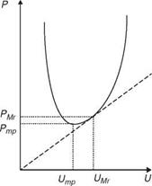
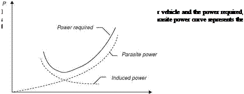
Figure 1.33. The U-shaped power curve for a fixed-wing aircraft. Ump is the velocity for minimumpower (Pmp) and UMr is the velocity for maximum range.

Figure 1.34. Comparative mass-specific pecto­ralis power as a function of flight velocity in cock – atiels, doves, and magpies. Bird silhouettes are shown to scale digitized from video [83].

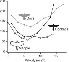Nevertheless, as shown in Figure 1.34, the L-shaped power-flight speed curve is indeed observed in natural flyers.

Can scaling arguments provide any information about limits on the size of flapping flyers capable of sustained flight? As mentioned earlier, large pterosaurs once flew long ago; some of these species were much larger than the birds of today. There are discussions about whether they were able to flap or only to soar [4]. There are many parameters to consider when flapping flight is studied, but limitations to this kind of flight mainly depend on the power available and structural limits.

These limitations are intimately connected, because flapping frequency affects both power and structural limits. To generate the power required for flight, most birds and other flapping animals have well-developed flight muscles. For birds these muscles are the pectoral muscles, which power the downstroke of the wings, and the supracoracoideus muscles powering the upstroke. Much effort has been made to determine power output and frequency levels and to compare the masses of these muscles with the mass of the whole specimen. According to Rayner [56], relations between body mass m and the mass of the pectoral and supracoracoideus muscles, mp and ms, respectively, can be expressed as

mp = 0.15 m099, (1-26)

ms = 0.016 m101. (1-27)

This means that the flight muscles constitute approximately 17 percent of the total weight. In comparison, the muscle of human arms accounts for about 5 percent of total body weight, according to Collins and Graham [76]. The power output from bird muscles and “fast” human muscles is about the same, 150 W/kg. Because the wings are often flexed during the upstroke and therefore not exposed to the same aerodynamic force or moment of inertia as during the downstroke, the weight of the supracoracoideus muscle is generally low compared with the weight of the pectoral muscle. Hummingbirds are different, having an aerodynamically active upstroke (producing lift). In their case, the weight of the supracoracoideus is higher; according to Norberg [4], this muscle group can constitute up to 12 percent of the body weight. The smallest supracoracoideus muscles are found among species with large wingspan, where the muscle mass is about 6 percent of the total mass. This value is comparable to that of the human body, and hence, these species have difficulties taking off without a headwind, running start, or a slope-start from a height. However, species with a long aspect ratio are usually able to soar, so the duration of the flapping flight mode can therefore be decreased.

Pennycuick [62] [77] [78] defined the power margin as the ratio of the power available from the flight muscles to that required for horizontal flight at the minimum power speed. As already mentioned, the power available depends on the flapping frequency, which determines the upper and lower limits of the size of flying animals. Pennycuick [78] concluded that the upper limit for flapping flight, based on actual sizes of the largest birds with powered flight, is a body mass of about 12 to 15 kg. Larger birds do not have the possibility of beating their wings fast enough to generate lift to sustain horizontal flight. Smaller birds have the advantage of being able to use different flapping frequencies, but for animals with a weight of about 1 gram, there is another upper limitation. Their muscles need time to reset the contractile mechanism after each contraction [4]. For insects with wing-beat frequencies up to 400 Hz, this problem is solved with special fibrillar muscles capable of contracting and resetting at very high frequencies. This limitation results in a minimum mass for birds of

1.5 grams and, for bats, 1.9 grams.

The upper and lower wing-beat frequencies are also restricted because of the structural limits. Bones, tendons, and muscles are not capable of performing wing motions above a certain wing-beat frequency. Wing bones that have to transmit forces to the external environment during flight must be strong enough to not fail under the imposed loads. This means that the bones have to be stiff and strong and at the same time not too heavy. Kirkpatrick [61] investigated the scaling rela­tionships between body size and several morphological variables of bird and bat wings in order to estimate the stress levels in their wings. He also estimated the bending, shearing, and breaking stresses in the wing bones during flight. He sug­gested that the breaking stress for a bat humerus bone is around 75 MPa and for birds 125 MPa. This structural limit helps explain why no bat weighs more than 1.5 kg. Kirkpatrick [61] found that no relationship exists between either bending or shearing stresses and wingspan during gliding flight and during the downstroke in hovering flight. In general, the safety factors are greater for birds than for bats. Hence birds are more capable of withstanding higher wing load­ing. A final conclusion by Kirkpatrick [61] is that the stresses examined are scale independent.

One of the first researchers to explore the consequences of the trend in which larger animals oscillate their limbs at lower frequencies than smaller ones of a similar type was Hill [72]. He concluded that the mechanical power produced by a particular flight muscle is directly proportional to the contraction frequency. This conclusion has made flapping frequency an important parameter when trying to describe the theories behind flapping wings. Pennycuick [73] conducted one of the most thorough studies of the wing-beat frequency. He assumed that there is a natural frequency, imposed on the animal by physical characteristics of its limbs and by the forces they have to overcome. To be efficient, locomotion muscles have to be adapted to work at a particular frequency. For example, for walking animals, Alexander [74] showed that the first natural frequency is proportional to

(1-21)

where g is the acceleration of gravity and Zleg the leg length. Similar approaches can be used for flight.

Pennycuick [73] identified several physical variables that affect the wing-beat frequency:

b: Wing span (m)

S: Wing area (m2)

I: Wing moment of inertia (kg m2) ~ m(b/2)2 p: Air density (kg/m3)

Allowing these variables to vary independently and assuming that the wing moment of inertia is proportional to m(b/2)2, Pennycuick [73] deduced the following correlation for the wing-beat frequency by incorporating data from 32 different species:

f = 1.08(m1/3g1/2b-1S,-1/4p1/3). (1-22)

In an updated study Pennycuick [59] added 15 species and made a more detailed analysis. This leads to the following expression:

f = m3/8g1/2b-23/24 S-1/3p3/8. (1-23)

Equation (1-21) can be used to predict the wing-beat frequency of species whose mass, wing span, and wing area are known. As mentioned earlier, the moment of inertia I for the wing is dependent on both the span b and the body mass m; hence, a change in any of these variables will result in a change in the moment of inertia. This effect may not be appropriate, given that a change in, for instance, body mass does not necessarily affect the number of the moment of inertia I. So, if we intend to predict these effects on the wing-beat frequency, it is more suitable to include I as an independent parameter [59]:

f = (mg)1/2 b-17/24S-1/31-1/8 p3/8. (1-24)

Another relation observed by Pennycuick et al. [75] is the effect of air speed on wing – beat frequency when body mass changes. The data for the wing-beat frequency and the air speed, U, are fitted with a least squares method:

f = k2 + k3/U + k4U3, (1-25)

where k2, k3, and k4 are proportional constants.

Whether a flying animal can hover or not depends on its size, the moment of inertia of its wings, the degree of freedom in the movement of the wings, and the wing shape. As a result of these limitations, hovering is mainly performed by smaller birds and insects. Larger birds can hover only briefly. Although some larger birds, such as kestrels, seem to hover more regularly, in fact they use the incoming wind to generate enough lift. The two kinds of hovering, symmetric and asymmetric, are described by Norberg [4] and Weis-Fogh [68].

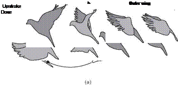
Because larger birds cannot rotate their wings between forward and backward strokes, they extend their wings to provide more lift during downstroke, whereas during the upstroke their wings are flexed backward to reduce drag. In general the flex is more pronounced in slow forward flight than in fast forward flight. This type of asymmetric hovering, usually called “avian stroke” [24], is illustrated in Figure 1.28. As shown, to avoid large drag forces and negative lift forces, these birds flex their wings during the upstroke by rotating the primaries (tip feathers) to let air through.

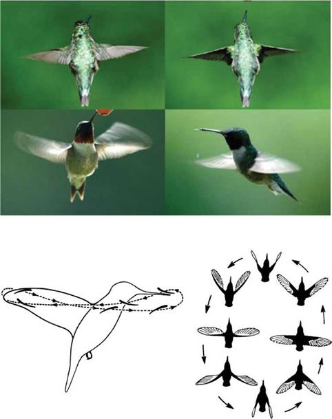
Symmetrical hovering, also called normal or true hovering, or “insect stroke,” is performed by hummingbirds or insects that hover with fully extended wings during the entire wing-beat cycle. Lift is produced during the entire wing stroke, except at the reversal points. The wings are rotated and twisted during the backstroke so that the leading edge of the wing remains the same throughout the cycle, but the upper surface of the wing during the forward stroke becomes the lower surface during the backward stroke. The wing movements during downstroke and upstroke can be seen in Figure 1.29. As shown, hummingbirds can rotate their shoulder joint enough to flip the wing over on the upstroke. Like most insects, they hover symmetrically with

0.01 sec intervals

(b)

Figure 1.27. Schematic sketches of the roles of the outer and inner wing (a) and the up – and downstroke (b) for bird flight. The outer wing area is the main source of weight support and thrust generation during the downstroke. During the upstroke the forces are minimized. Upstroke is suitable for a small amount of thrust in slow flight, but not much weight support.

a horizontal stroke plane. Their supracoracoideus (pull the wing down) is half the size of the pectoralis (pull the wing up). Note that, during hovering, the body axis is inclined at a desirable angle and the wing movements describe a figure-eight pattern lying in the vertical plane.

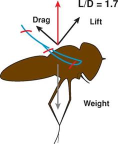
Most birds and bats hover with the stroke plane inclined about 30 degrees to the horizontal. As illustrated in Figure 1.30, the resultant downstroke force with a

lift-to-drag ratio of 1.7 is vertical. Except for small species, noticeably hummingbirds, the wing is typically flexed on the upstroke, minimizing forces on the wing. In inclined hovering flight, lift and drag on the downstroke support the weight.

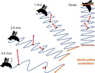
Figure 1.31 illustrates the wing paths and associated kinematics at different speeds of a bumblebee flying at varying flight speed. The wings flap in a stroke plane

and flip over between half-strokes, resulting in forces that are nearly symmetrical in hovering. As the forward speed increases, the force generation between the up – and downstrokes becomes progressively different in magnitudes, with the downstroke becoming more dominant.