Let u(t) represent a random function of time, such as a velocity component at a point in a turbulent flow, the force acting in the landing-gear strut of an airplane during landing impact, the lift acting on an airfoil in passing through a gust, etc. By saying that u(t) is a random function, we mean that at a given time t the value of и is not predictable from the data of the problem but takes random values which are distributed according to certain definite probability laws. We shall assume that the probability laws describing the randomness are determined by the data of the problem. Such a determination can sometimes be made through a suitable theoretical model, but in general it has to be obtained by experiments.
A set of observations forms an “ensemble” of events. In the example of gusts, each gust record, such as the one given in Fig. 8.6, is a member in an ensemble of such records. Imagine that a large number of observations be made simultaneously under similar conditions. Let the records be numbered and denoted by uft), u2(t), • • •, uN(t). If the total number of records is N, the following averages may be formed
/wwvjV
u{t) = [uft) + «2(0 + ‘ ‘ • + uN(t)]/N
www’ r
ut) = Wit) + «до + • ■ • + uNt)W (l)
Assume that «(/) and ut) , etc., tend to definite limits, respectively, as N -> 00; then these limiting values are ensemble averages of the random process «(0-
In a similar manner, ensemble averages of the following nature can be formed:
N
^WVWV ллл/wv J ^
u{t)u{t + t) = lim — > «ДК(г + т) (2)
2V—>cc -/V
г = 1 N
u(t)u(t + rx) ■ ■ ■ u(t + rm) = lim — / «г(0«;0 + Tj) • • • U,{t + Tm)
ДГ-*0О A Z—t
г = 1 (О
These are ensemble averages of the correlation functions of the random function u(t).
For a complete statistical description of a random process, ensemble averages of all orders are required. However, for practical dynamic-load problems in aeroelasticity, often the most important information is
TRANSIENT LOADS, GUSTS
ЛАЛЛ VWVW J
afforded by the mean value u(t) and the mean “intensity” (ut)) For
these simplest kinds of average quantity, analysis can proceed in a simple
manner. By definition, it is clear that u(t) and ([«(r) — м(Г)]2)1/г are the mean and the standard deviation of the random function u{t) at any instant t.
If the ensemble averages of a function u(t) are independent of the variable t, then u(t) is said to be stationary in the ensemble sense.
A different kind of average is the well-known concept of time average. Thus, the mean and the mean square of a function of time u(t) over a time interval 2T, are
|
—- T
|
1
|
П+Т
|
|
u{t)
|
“ 2T.
|
u(t) dt
It —T
|
|
1 і
|
ft + T
|
|
ut)
|
= 2rJ
|
ut) dt
l – T
|
Similarly, higher-order averages u%t) (p = 3, 4, • • •) can be formed,
provided that the definition integrals converge. If the time averages tend
to be independent of t and T when T is sufficiently large, then u(t) is also
said to be stationary, but in the sense of time-average. We shall write in
____ 2′ ………………………….
this case the limiting value of uv{t) as T > oo as up(t).
The property of stationariness says, in effect, that all time instants are similar as far as the statistical properties of и are concerned. This suggests that the results of averaging over a large number of observations could be obtained equally well by averaging over a large time interval for one observation. In other words, for a stationary random process, one expects the time averages to be equal to the ensemble averages, and we do not have to distinguish the concepts of stationariness in time average or in ensemble average. The study of the exact conditions under which this equivalence of the time average over one observation and the ensemble average over many observations will indeed be true is called the ergodic theory. In aeroelastic problems which we are going to consider, this equivalence may be assumed.
It is natural to extend the above concepts to random functions of space. In the example of gusts, we may have to consider the velocity fluctuation u, itself a vector, as a function of space and time x, y, z, t. If records of the velocity fluctuation were taken over different regions of space and if the ensemble averages over space are independent of the spatial coordinates of the regions, then the velocity fluctuation is said to be homogeneous.
There are many flows, of interest to aeroelasticity, that are approximately homogeneous and stationary when the time and distance scales
are properly chosen. Such is the case of atmospheric turbulence within a suitable expanse of time and space.
The Power Spectrum. Let us consider a stationary random process u(t) which has a mean value m equal to zero[23] and define the mean square of u(t) over an interval 2T as in Eq. 4. Let u(t) be so “truncated” that it becomes zero outside the interval (— T, T) (Fig. 8.8). Let the truncated function be written as uT(t).
|

Fig. 8.8. A truncated function.
|
The Fourier integral of uT(t) exists provided that the absolute value of uT(t) is integrable and uT(t) has bounded variation,
uT(t) = –== f FT(co) еІШІ dco (5)
V2lT J – со
where
FT(co) = —U Г uT(t) e~imt dt (6)
v2tt J-t
If FT*(co) denotes the complex conjugate, then FT*{— со) == FT(co) since uT(t) is real. It is well known (Parseval theorem) that
f uT2(t) dt = f uT2(t) dt = f FT(co)2 dco (7)
J— oo J — T J— да
Hence
___ 1 Гда /*да <sr (fjy)|2
ut) = lim — FT (со) 12 dco = lim —^——– dco (8)
r—>co сіл J —со T—> CO 00 Z
For a stationary random process for which u2(t) exists, the left-hand side of the above equation tends to a constant as T oc; hence let
|
p(m) – lim
(ZWoo 1
|
(9)
|
|
C oo
|
|
u2(t) — p(m) dm Jo
|
(10)
|
The function p(oj) is called the power spectrum or the spectral density of u(t). When u{t) is resolved. into harmonic components by a Fourier analysis, as in Eq. 5, the element p(co) dm gives the contribution to u2(t) from components having frequencies ranging from m to c/j + dm. The integral
/•to
p(m) dm represents the contribution to u2(t) from frequencies less than m. Jo
Correlation Functions. Consider again a stationary random process u(t), and define the average value
—————- 1 Г
W(t) = «(0 u(t + t) = lim —; u(t) u(t + t)dt (11)
37—► oo і J — T
ір(т) as a function of т is a correlation function defined in the sense of time average. For a stationary random process it is the same as that defined in Eq. 2.
It follows from the definition of correlation function that
№ = Ш (12)
Since the average values of a stationary random process are independent of the origin of t, it follows immediately that
УІт) = У (— r) (13)
Furthermore, if u(t) is a continuous function of t, then
lim u(t)[u(t + t + h) — u(t + t)] = 0
Й-И)
since the factor in [ ] tends to zero as h -> 0. This may be written as
lim [tp(r + h) — y<t)] = 0 (14)
A->0
showing that ір(т) is continuous at all values of t. According to the Schwarzian inequality,
y(r) < [u2(t) • u2(t + r)]1’2 = [?/>(0) • W(0)p‘
we have
In general, random processes having zero mean values satisfy the condition
lim yj(r) = 0 (16)
T—> CO
which means that the function «(/) at two instants separated by a long time interval are uncorrelated with each other.
The correlation function y(r) when plotted against r is generally a bellshaped curve. The interval of т in which y(r) differs significantly from zero is a measure of the “scale” of the random process. In the example of atmospheric turbulence, such a scale may be thought of as representing the mean size of eddies.
Relation between the Power Spectrum and the Correlation Function. The Fourier transform of y(r) is
ф(а>) = -)= Г w(T)e-imrdr (17)
V2lT J – 00
Since y(r) is an even function of т, ф(со) can be expressed as a real-valued integral
/2 Г®
ф{со) — ^ — J y(r) cos сот (It
because е~ыЛ = cos сот — г sin сот and the imaginary part of Eq. 17 vanishes. The inverse transform is –
І2 f®
w(t) — – ф(со) cos сот dco
^ – it Jo
When t 0, the left-hand side tends to ut); hence
m[24](0 =J – Ф(ю) dco
A comparison with Eq. 10 shows that, aside from the numerical factor V2/77, ф(со) is identical with the power spectrum p(co) defined before. A formal proof for the identity of ^ — ф(со) with p(co) can be constructed.
Hence, we obtain the reciprocal relations between the power spectrum and the correlation function
Equations 5 through 19 hold for any stationary function u{t). Now consider an ensemble of functions и ft), и ft), ■ • •. Each of these functions defines its p{m) and ір(т), which can be averaged over the ensemble.
The resulting p(co) will be called the spectral density or the power spectrum of the random process. For a stationary random process it follows from Eqs. 18 and 19 that the correlation function and the power spectrum are each other’s Fourier cosine transform.
Example. When
y(t) = A + В sin (ay + °0
we have
У2 = A2 + B2
w(T) = + t) = A2 +B2 cos ay
and, if we define a unit-impulse function 6(t) as in Eq. 14 of § 8.1, but
Л OO
impose further the condition d(t) — <5(— t) so that 6(t)dt — then
Jo
p(co) = 2A2d(co) — 132S(oj — co0)
This example shows that, if the mean value of a function is not zero, and if the function is periodic, the power spectrum will have singular peaks of the well-known Dirac й-function type.
Example of Wind-Tunnel Turbulences. Consider the velocity fluctuations in the flow in a wind tunnel. Let the deviations from the respective mean values of the velocity components be written as иъ u2, u3. These are functions of space and time (x, y, z; t). Similar to the time correlation function гр(г), the spatial correlation functions such as
Щ(х, у, z; t)u3(x + r, y,z;t)
1 Г (20)
= lim — щ(х, у, z; t)u,(x + r, y,zt) dx dy dz (i, j =1,2, 3)
F->co r JV
may be formed. If the field of flow is homogeneous, such a correlation function is well defined and is a function of r and t only. It is possible in wind-tunnel work to determine experimentally the general correlation function
Щ(хъ уъ 2X; t^ufxi, уг, z2; t2) (/, j = 1, 2, 3) (21)
which, for a stationary and homogeneous turbulence field, depends only on the relative position of the points (aq, ylt Zj) and (x2, y2, z2), and the time interval t2 — tx, and not on the absolute location of the points or time.
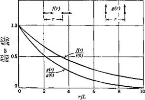
Thus a large number of space and time correlation functions can be defined among various velocity components. It is here that the simplifying concept of an isotropic turbulence field enters. As was first shown by G. I. Taylor8 54 and Th. von Karman,8-51 an isotropic turbulence field is one that can be specified by two “principal” velocity correlations, in a way similar to that two principal stresses at a point in an isotropic elastic solid define the state of stress at that point. The two principal velocity correlations are denoted by / and g and are defined pictorially in Fig. 8.9. /(/•) is the correlation function between the same velocity component measured at two points at a distance r apart, lying along a line in the direction of the velocity component. g(r) is the correlation function between points at a distance r apart, lying along a direction normal to the direction of the velocity component. For example, let us write u, v, w in place of иъ иг, щ, then
u(x, y, г; t)u(x + r, y,z;t) = /0)
 u(x, y, 2; t)u(x, у + r, z;t) = g(r)
v(x, y, 2; t)v(x + r, y,z;t) = g(r)
If the field of fluctuation u, v, w is superimposed upon a mean flow of velocity U is the x direction, and if к2/!/2, t>2/ C/2, w2/t/2 are small quantities, it is possible to interchange time and space variables and consider the turbulence as simply being transported along with the velocity U in the x direction. Hence the time т which enters into the time correlation function can be replaced by r/С/, where r is chosen along the x axis. We may write
 u(t)u(t + t) = xp-tir) = f(rU)
v(t)v(t + т) = У’2(т) = g(jU)
Experiments8-1 have shown that in wind-tunnels the turbulences are nearly isotropic and the correlation functions f(r) and g(r) have the form

(24)
|

Fig. 8.9. Correlation functions / and g in isotropic turbulences.
|
|
 |
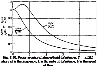
and the power spectra are
AH =A(°)
 1 + 3f2a аИ=М°)(ГТ1^
where
The functions fir), g(r), and p2(oi) are normalized and depicted in
Figs. 8.9 and 8.10.
|
The constants by and L2 in the above equations are quantities known as scales of turbulence. They are proportional to the areas under the normalized correlation curves
|
|
|
|
Consider a very simple experiment of tossing a coin and observing whether a “head” turns up. If we make n throws in which the “head” turns up v times, the ratio vjn may be called the frequency ratio or simply the frequency of the event “head” in the sequence formed by the n throws. It is a general experience that the frequency ratio shows a marked tendency to become more or less constant for large values of n. In the coin experiment, the frequency ratio of “head” approaches a value very close
to Vs-
This stability of the frequency ratios seems to be an old experience for long series of repeated experiments performed under uniform conditions. It is thus reasonable to assume that, to any event £ connected with a random experiment S, we should be able to ascribe a number P such that, in a long series of repetitions of S, the frequency of occurrence of the event E would be approximately equal to P. This number P is the probability of the event E with respect to the random experiment S. Since the frequency ratio must satisfy the relation 0 < vjn < 1, P must satisfy the inequality
0 < P < 1 (1)
If an event E is an impossible event, i. e., it can never occur in the performance of an experiment S, then its probability P is zero. On the other hand, if P = 0 for some event E, E is not necessarily an impossible event. But, if the experiment is performed one single time, it can be considered as practically certain that E will not occur.
Similarly, if £ is a certain event, then P = 1. If P = 1, we cannot infer that £ is certain, but we can say that, in the long run, £ will occur in all but a very small percentage of cases.
The statistical nature of a random variable is characterized by its distribution function. To explain the meaning of the distribution function, let us consider a set of gust records similar to the one presented in Fig. 8.6. Let each record represent a definite interval of time. Suppose that we are interested in the maximum value of the gust speed in each record. This maximum value will be called “gust speed” for conciseness and will be denoted by y. The gust speed varies from one record to another. For a set of data consisting of n records, let v be the number in which the gust speed is less than or equal to a fixed number x. Then vjn is the frequency ratio for the statement у < x. If the total number of records n is increased without limit, then, according to the frequency interpretation of probability, the ratio v/n tends to a stationary value which represents the probability of the event “y < x.” This probability, as a function of x, will be denoted by
P(y^x) = F(x) (2)
The process can be repeated for other values of x until the whole range of x from — oo to oo is covered. The function F(x) defined in this manner is called the distribution function of the random variable y.
Obviously F(x) is a nondecreasing function, and
F(- oo) = 0, 0 < F(x) < 1, F(+ oo) == 1 (3)
If the derivative F'(x) — f(x) exists, fix) is called the probability density or the frequency function of the distribution. Any frequency function f{x) is nonnegative and has the integral 1 over (— oo, oo). Since the difference Fib) — F(a) represents the probability that the variable у assumes a value belonging to the interval a <y < h,
P(a < у < b) = F(b) – F(a) (4)
In the limit it is seen that the probability that the variable у assumes a value belonging to the interval
x < у < x + Ax
is, for small Ax, asymptotically equal to f(x) Ax, which is written in the usual differential notation:
P(x < у < x + dx) — f(x) dx
In the following, we shall assume that the frequency function fix) = F’ix) exists and is continuous for all values of x. The distribution function is then
if absolutely convergent, are called the first, second, third, • • ■ moment of the distribution function according as v = 1, 2, 3 • • • respectively. The first moment, called the mean, is often denoted by the letter m
m = f хДх) dx (8)
J — oo
The integrals
Л 00
Uv = I (x — mf f(pc) dx (9)
J — CO
are called the central moments. Developing the factor (x — my according to the binomial theorem, we find
fi0 = 1
^i = 0
/4 2 = <*2 — (50)
ys = «з — 3ma2 + 2 rtf
Measures of location and Dispersion. The mean m is a kind of measure of the “location” of the variable y. If the frequency function is interpreted as the mass per unit length of a straight wire extending from — oo to – f oo, then the mean m is the abscissa of the center of gravity of the mass distribution.
The second central moment gives an idea of how widely the values of the variable are spread on either side of the mean. This is called the variance of the variable, and represents the centroidal moment of inertia of the mass distribution referred to above. We shall always have > 0. In the mass-distribution analogy, the moment of inertia vanishes only if the whole mass is concentrated in the single point x = m. Generally, the smaller the variance, the greater the concentration, and vice versa.
In order to obtain a characteristic quantity which is of the same dimension as the random variable, the standard deviation, denoted by a, is defined, as the nonnegative square root of
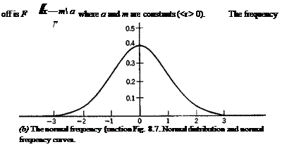
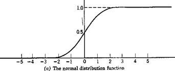
The corresponding normal frequency function is
f(x) = – l=e-*al* (13)
V 27Г
Diagrams of these functions are given in Fig. 8.7. The mean value of the distribution is 0, and the standard deviation is 1.
A random variable f will be said to be normally distributed with the parameters m and a, or briefly normal (m, a) if the distribution function

F(x)
|

f(x)
|
function is then
  (14) (14)
It is easy to verify that m is the mean, and a is the standard deviation of the variable f.
Note that, in the normal distribution, the distribution function is completely characterized by the mean and the standard deviation.
| |


