Our heavyweight helicopter equal in the world does not have
In Rostov started production of the most load-lifting rotary-wing car The Russian holding «Helicopt[...]

Everything about aircrafts and helicopters. News and events in aviation worldwide. Civil, transportation, military helicopters and airplanes.

Everything about aircrafts and helicopters. News and events in aviation worldwide. Civil, transportation, military helicopters and airplanes.

Everything about aircrafts and helicopters. News and events in aviation worldwide. Civil, transportation, military helicopters and airplanes.

Everything about aircrafts and helicopters. News and events in aviation worldwide. Civil, transportation, military helicopters and airplanes.


At zero degree angle of attack, the computed boundary layer flow on the airfoil remains attached almost to the trailing edge. The boundary layer flow is steady while the flow in the wake is oscillatory. Figure 15.31 shows a plot of the computed instantaneous vorticity field around Airfoil #2 at a Reynolds number of 2 x 10⁵.
The leading edge of the airfoil is placed at x = 0. This is typical of all the cases investigated. The flow leaves the trailing edge of the airfoil smoothly. There is no vortex shedding at the trailing edge, regardless of previous speculation (Paterson et al., 1973). The oscillations in the wake intensify in the downstream direction until it rolls up to form discrete vortices further downstream.
Figure 15.32 shows an instantaneous streamline pattern of the wake of Airfoil #2 at a Reynolds number of 4 x 10⁵. The wake oscillation is prominent in this figure. The wavelengths of the oscillations appear to be fairly regular. This suggests that there is flow instability in the wake.
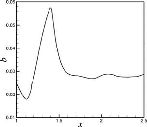
The mean velocity deficit profile in the wake resembles a Gaussian function. The half-width of the wake, b, near the airfoil trailing edge undergoes large variation in the flow direction. Figure 15.33 shows the variation of the half-width as a function of downstream distance for Airfoil #2 at a Reynolds number of 2 x 10⁵. The width of the wake begins to shrink right downstream of the airfoil trailing edge until a
 |
Figure 15.33. Spatial distribution of the half-width of the wake for Airfoil #2 at Re = 2 x 10⁵.
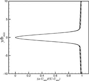
Figure 15.34. Similarity of velocity deficit profile at b = bmin in the wake of Airfoil #2. Reynolds number varies from 2 x 10⁵ to 5 x 10⁵ at 0.5 x 10⁵ interval.
 minimum is reached at b = bmin. It grows rapidly further downstream, reaching a maximum before decreasing and attaining a nearly asymptotic value.
The velocity deficit profiles of the wake exhibits self-similarity. Figure 15.34 shows a collapse of the velocity profiles at minimum half-width over a large range of Reynolds numbers. In this figure, the variable (u – Umin)/(U – Umin) is plotted against y/bmin, where Umin is the minimum velocity of the mean flow profile and b is the half-width. In Figure 15.34, data from Reynolds number of 2 x 10⁵ to 5 x 10⁵ at 0.5 x 10⁵ intervals are included. There is a nearly perfect match of the set of seven profiles.
The similarity property of the wake velocity profiles suggests the possibility of the existence of a simple correlation of the minimum half-width of the wake with flow Reynolds number (Re). Figure 15.35 shows a plot of (bmin/C)Re1/2 against Re (C is the chord width) for Airfoil #2. It is seen that the measured values of this quantity from the numerical simulations are nearly independent of Reynolds number over the entire range of Reynolds number of the present study. Thus, the minimum halfwidth of the wake, bmin, of Airfoil #2 has the following form of Reynolds number dependence:
A similar analysis has been performed for Airfoil #1. Figure 15.36 shows that the quantity (bmin/C)Re1/2 again is approximately a constant. In this case, the value bmin and Reynolds number are related by,
b 1
-^Re^ «7.45. (Airfoil #1). (15.57)
To ensure a numerical simulation has adequate resolution, ideally, grid refinement should be performed. Essentially, one would like to show that the computed results are grid size independent. However, for large-scale simulation this is not always feasible. Often, this is because of the complexity of the computer code. Another reason is that some simulations may require exceedingly long computer run time. This invariably discourages the performance of grid refinement. For the airfoil tone simulations, it is a medium-size simulation so that grid refinements in relation to the numerical results discussed below have been carried out. In the grid refinement exercise, all the mesh sizes in the elliptical region of the computational domain are reduced by half. Two test cases are chosen with Reynolds numbers equal to 2 x 10⁵
 |
and 4 x 10⁵. For the low Reynolds number case, the tone frequency is found to remain essentially the same. For the higher Reynolds number case, the tone frequency reduces by 2 percent with the finer mesh. On assuming that the difference is proportional to the Reynolds number of a simulation, it is estimated that the numerical results should be accurate to about 3 percent for the highest Reynolds number simulations.
15.4.1 Numerical Results
A computer code based on the methodologies described above has been developed. The code is then used to investigate airfoil tones of three NACA0012 airfoils with truncated trailing edges as proposed in Section 15.3.3. The dimensions and trailing edge thicknesses of the airfoils are given in Table 15.2. The trailing edge profiles of these airfoils are shown in Figure 15.30.
In this study, the original airfoil chordwidth is 0.1 m. The airfoil is placed in a uniform stream with a velocity U. The Reynolds number range of the present study is from 2 x 10⁵ to 5 x 10⁵. For a flat plate with the same length, the displacement thickness at the trailing edge at Reynolds number of 2 x 10⁵ is S* = 1.72(Cu/U)2 = 3.85 x 10⁻⁴ m. Thus, RS* is equal to 770. For this Reynolds number, the wake flow is laminar in the absence of high-level ambient turbulence. In the present simulations,
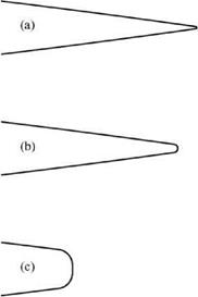 Figure 15.30. Trailing edge profiles of the three NACA0012 airfoils under study. (a) 0.5 percent truncation, (b) 2 percent truncation, (c) 10 percent truncation.
 |
this remains true even at the highest Reynolds number of the study. However, it may not be true for the three-dimensional simulation. In this study, the angle of attack is set at zero degree. This is to keep the flow and, hence, the tone generation as simple as possible. At a high angle of attack, separation bubble and open separation often occur on the suction side of the airfoil. Under such conditions, other tone generation mechanisms may become possible, but this is beyond the scope of this study.
 |
|
The governing equations are the dimensionless Navier-Stokes equations in two dimensions and the energy equation. Here, the length scale is C (chord width), velocity scale is aO (ambient sound speed), time scale is C/aO, density scale is pO (ambient gas density), pressure and stress scales are pOaO. These equations are as follows:
U is the free stream velocity, M is the Mach number, Re is the Reynolds number based on chord width. Both viscous dissipation and heat conduction are neglected in the energy equation as the Mach number is small.
The time step used in the computation is selected to meet the stability and accuracy requirements of the subdomain with the smallest size mesh. In the computation domain, the governing partial differential equations have variable coefficients. It is impractical to perform numerical stability analysis for equations with variable coefficients. Here, the frozen coefficient approximation is invoked. Under this approximation, the coefficients are treated as constants. To further simplify the analysis, the viscous terms that are diffusive in nature will be neglected. In the д – в plane, the linearized governing equations are Eq. (5.61), which may be written in the following form:
![]()
|
where
|
p" |
иДх + V py |
PPx |
PPy |
0 |
|
|
и |
, a = |
0 |
иДх + V py |
0 |
Px/p |
|
v |
0 |
0 |
U^x + V^y |
PyfP |
|
|
P- |
0 |
Y pPx |
Y PPy |
Upx + VPy |
|
u |
|
x |
![]() В
В
where subscripts x and y indicate partial derivatives. u, v, p, and p are local values. Coefficient matrices A and В are to be regarded as constants in the analysis.
Numerical stability analysis follows the procedure of Section 5.3. For this purpose, the Fourier-Laplace transform is applied to Eq. (15.49) locally. The Fourier- Laplace transform in the p – O plane is defined by
TO
U(а, в,а>) = ^2^3 j j j u(p, O, t) e—l(ap+eo—mt) dp de dt.
— TO
The Fourier-Laplace transform of Eq. (15.49) is
0 ю — (a u + P v) 0 — a/p
![]()
0 0 ю — (a u + P v) —P /p
0 — y pa — – pP ю — (au + j3v) where a = a/лх + вд p = aQx + вQy. The eigenvalues of matrix К are as follows:
■1 = ■Ч = [ю — (au + p v)]
■3,4 = ю — (au + Pv) ± (yp/p)1/2(a2 + P2)1/2.
The dispersion relation that imposes the most stringent stability requirement is that of the acoustic wave Л4 = 0. On proceeding as in Section 5.3, it is straightforward to derive the following maximum time step formula should the 7-point stencil DRP scheme be used for the computation.
15.4.1.2 Starting Conditions
In the course of performing the airfoil tone simulations, it has been found that the following simple starting conditions have been very successful:
1
t = °, u = ^incoming, v = 0> Р = 1 P = -•
The uniform starting condition is applied throughout the entire computational domain. In order to comply with the no-slip boundary conditions on the airfoil surface, the boundary conditions on the airfoil surface, д = 0, is taken to be
Here, t is recommended to be five or six times of the tone period. The no-slip boundary conditions are attained at t = T.
The addition of artificial selective damping is absolutely necessary when a central difference time marching scheme is used for computation. A central difference scheme has no intrinsic damping. It has to rely on artificial damping to eliminate spurious waves and to maintain numerical stability. To eliminate spurious waves requires background damping over the entire computational domain. The idea is to damp out spurious waves as they propagate across the computational domain. The
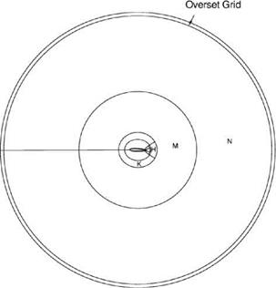 Figure 15.27. Subdomains H, K, M, and N in physical space.
damping terms to be added to the governing equations in the computation plane has the following form:
d U 1 , / ч _
TT7 + = – „ djui+jm + ui, m+j), (15.46)
dt j=-3
where t is nondimensionalized by А/л/a. RA/x is the mesh Reynolds number as discussed in Chapter 7.
To maintain numerical stability, a very different strategy is required. Spurious waves are often generated and amplified at boundaries and surfaces of discontinuities. They include solid surfaces, external boundaries of a computational domain, and mesh-size-change interfaces. To suppress the generation and amplification of spurious waves, especially grid-to-grid oscillations, extra damping is imposed along narrow strips of the computational domain bordering the boundaries and surfaces of discontinuities.
Background damping is usually imposed through the use of the damping curve with a half-width a = 0.2n (see Section 7.2). This damping curve targets the high wave numbers of the spectrum and introduces minimal damping to the low wave numbers. The amount of damping imposed is specified by the value assigned to the inverse mesh Reynolds number RAX = (a0A/va)-1. A recommended value to use is Ra1 = 0.05. The artificial selective damping stencil is designed to automatically adjust to the mesh size used, so there is no need to make provision to adjust the value of Ra1, because of the different mesh size used in different subdomains.
Near a surface of discontinuity such as a wall, a typical stencil arrangement is to impose extra damping as shown in Figure 7.7. Since all damping stencils are symmetric, the first mesh points to apply artificial selective damping are those on the first row immediately away from the surface of discontinuity. Here, a 3-point damping stencil is used. For the next row of mesh points, a 5-point damping stencil is used. For the third mesh row from the surface of discontinuity and for mesh points further away, a 7-point damping stencil is used. In the direction parallel to the surface of discontinuity, a 7-point damping stencil is used whenever possible. The damping curve with a half-width equal to 0.3n (see Section 7.2) would be most appropriate. To make sure damping is confined to a narrow strip adjacent to the surface of discontinuity, the inverse mesh Reynolds number is taken to be a Gaussian function centered on the surface of discontinuity. Specifically, if d is the distance of a mesh point from the surface of discontinuity, then it is recommended to take the inverse mesh Reynolds number at that point to be
— = Ae-(in2)(d/KA)2, (15.47)
ra
where for the airfoil tone problem, A is taken to be 0.1 and к, which controls the width of the damping strip, is usually set equal to 3 or 4. For the problem at hand, к is assigned the value of 4.
Near a sharp corner of a surface of discontinuity, additional damping is recommended. This is accomplished by adding an extra artificial selective damping term
Figure 15.28. Extra damping at the corner of two subdomains with different – size meshes.
 to the equations of motion. Let the coordinates of the corner point be (д0, в0), the inverse mesh Reynolds number of the extra damping term is taken to be
= £e-(ln2)[>-^0 )2+(в-в0 )2]/(кА)2, (15.48)
ra
where A2 = (Ад2 + Дв2). The extra damping imposed at a corner point of a mesh size discontinuity is illustrated in Figure 15.28.
For the airfoil problem, the distribution of extra damping is shown in Figure 15.29. According to this figure, extra damping is added along the surface of the airfoil and along mesh-size-change boundaries. Additional damping is used at corner points. At the overset grid region, extra damping is applied to the mesh points just inside the д = д^ boundary, where д^ is the largest value of д in the computational domain. No extra damping is imposed outside in the Cartesian grid domain.
For time marching computation in the elliptic coordinates region of the computational domain, Eqs. (15.42) to (15.45) are first rewritten in the д – в coordinates as in Section 5.6. The derivatives are then discretized according to the 7-point stencil DRP scheme. At the mesh-size change boundaries, the multi-size-mesh multi-time-step
DRP scheme of Chapter 12 is implemented. This scheme allows a smooth connection and transfer of the computed results using two different size meshes on the two sides of the boundary. It also allows a change in the size of the time step (see Figure 15.25). This makes it possible to maintain numerical stability without being forced to use very small time steps in subdomains where the mesh size is large. This results in a very efficient computation without loss of accuracy as noted in Chapter 12.
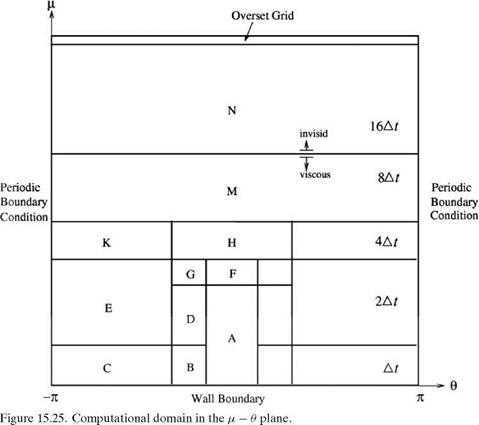 |
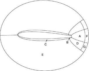
Figure 15.26. Various subdomains in the physical space.
On the left, the top and bottom boundaries of the computation domain shown in Figure 15.24, the radiation boundary conditions of Section 6.5 are imposed. On the right boundary, outflow boundary conditions of Section 6.5 are enforced. On the airfoil surface, the no-slip boundary conditions are used. This, however, will create an overdetermined system of equations if all the discretized governing equations are required to be satisfied at the boundary points. To avoid this problem, the two momentum equations of the Navier-Stokes equations are not enforced at the wall boundary points. The continuity and energy equations are, nevertheless, computed to provide values of density, p, and pressure, p, at the airfoil surface. This way of enforcing the no-slip boundary conditions was discussed at the end of Section 6.7.
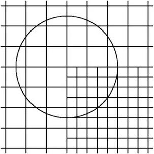
A well-designed grid is crucial to an accurate numerical simulation. For flow past an airfoil, accurate resolution of the boundary layer and wake flow is very important. To be able to do so, the use of a body-fitted grid is most advantageous.
The problem at hand is a multiscales problem. The smallest length scale of the problem that needs to be resolved is in the viscous boundary layer and in the wake. In this work, a multisize mesh is used in the time marching computation. Figure 15.24 shows the overall computational domain. It extends to a distance of 10 chordlengths in front of the leading edge of the airfoil and 30 chords downstream. The lateral dimension is 20 chords. The reason for choosing such a large computational domain is to provide sufficient distance for the wake flow and vortices to develop fully and to decay sufficiently before exiting the outflow boundary. A body-fitted elliptic coordinate system (p,, в) and mesh, as discussed in the Section 15.3, is used around the
|
Figure 15.24. Computational domain in physical space for uniform flow past an airfoil. |
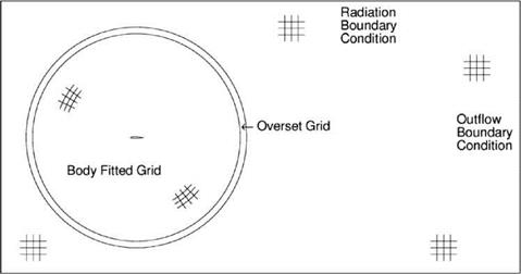
airfoil. This region extends to a radius of 8 chords (for large д, the elliptic coordinate system evolves into a polar coordinate system). Outside this nearly circular region, a Cartesian grid is used. This is illustrated in Figure 15.24. An overset grid region is created to encircle the body-fitted mesh. It is used to transfer computational information between the Cartesian grid and the body-fitted grid. The overset grid method of Chapter 13 is implemented here.
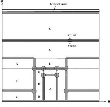
The boundary layer flow adjacent to the airfoil and the wake flow are believed to be responsible for the generation of airfoil tones. It is, therefore, important to provide sufficient spatial resolution in computing the flow in these thin shear layers. For this reason, in the grid design, the smallest size meshes are assigned to these regions. The grid layout in the д – в plane (the computational domain for the elliptic coordinate region) is as shown in Figure 15.25. In this figure, the range of в is from – n to n with periodic boundary conditions imposed on the left and right boundaries. The airfoil surface is on the line д = 0. This computational domain is divided into seventeen subdomains, symmetric about the line в = 0. The subdomains are labeled by a capital letter “A,” “B,” “C,” etc. In the physical plane, these subdomains are shown in Figures 15.26 and 15.27. Subdomains “B” and “C” contain the boundary layer. Subdomains “A” and “D” contain the near wake. Subdomains “F,” “H,” and “M” contain the intermediate wake. The far wake is in subdomain “N.” Subdomain “N” extends to the edge of the Cartesian grid region. Table 15.1 provides the mesh size assigned to each of the computational subdomains with Дв0 = 0.00218 and Дд0 = 0.0015. The mesh size of the Cartesian grid is uniform with Дх = Ду = 0.053.
15.4.1.1 Computational Model
In this study, a computational model consisting of a NACA0012 airfoil at zero angle of attack is used. The chord width, C, is 0.1 m, but the sharp trailing edge is truncated and fitted with a round trailing edge. The airfoil is placed in a uniform stream with a velocity Uranging from 30 m/s to 75 m/s. The kinematic viscosity of air, v at 15°C, is taken to be 0.145 x 10⁻⁴ m2/s. The corresponding Reynolds number, based on chord width, varies from 2 x 10⁵ to 5 x 10⁵.
The governing equations are the dimensionless Navier-Stokes equations in two dimensions. Here the length scale is C (chord width), velocity scale is aTO (ambient sound speed), time scale is C/aTO, density scale is p(ambient gas density), pressure and stresses scale is p^a^. These equations (in Cartesian tensor subscript notation) are
U is the free stream velocity, M is the Mach number, and Re is the Reynolds number. Both viscous dissipation and heat conduction are neglected in the energy equation. Away from the airfoil, viscous effects are unimportant. In this part of the computational domain, viscous terms are dropped, that is, the Euler equations replace the Navier-Stokes equations as the governing equations.
A very famous series of airfoil shapes is the NACA four-digit airfoils. These airfoils are completely defined by four parameters:
C the length of the chord line; є the maximum camber ratio;
p the chordwise position of the maximum camber ratio; t the thickness ratio (maximum thickness/chord).
If x is the distance along the chord, the thickness distribution is
 |
|
and the camber line (see Figure 15.18) is given by two parabolas joined at the maximum camber point as follows:
The first of the airfoil’s four-digit designation is 100e, the second digit is 10p, and the last two are 100т.
 |
|
The upper part of the airfoil is given by
Theoretically, one may have airfoils with sharp trailing edges. In reality, a sharp trailing edge is nearly impossible to make. Practical airfoils invariably have a blunt or slightly blunt trailing edge. A simple way to incorporate a blunt trailing edge to an airfoil is to replace the sharp tip by a semicircular arc as shown in Figure 15.19.
Figure 15.19. Blunt trailing edge of an airfoil.
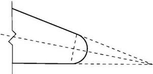
Analytically, for x > qc (q is the chordwise position of the circular arc), a blunt trailing edge airfoil has a thickness T and a camber line Y as follows:
Y(x) = Y'(qC)(x – qC) + Y(qC) (15.39)
However, the airfoil is slightly shortened. The new chord length is given by
C* = qC + r. (15.40)
2[1 + (Y’ (qC ))2]2
15.3 Example I: Direct Numerical Simulation of the Generation of Airfoil Tones at Moderate Reynolds Number
It is known experimentally that an airfoil immersed in a uniform stream at moderate Reynolds number would emit tones. This phenomenon has been studied by a number of investigators. Surprisingly, there are significant differences in their experimental results. Furthermore, there is no clear consensus on the tone generation mechanism. There are two objectives in including this problem in this chapter. The first objective is to demonstrate how to develop a CAA code. The second objective is to illustrate how direct numerical simulation can assist in resolving or clarifying experimental disagreement. In addition, numerical simulation provides a full set of space-time data (not always available from an experiment), which may be used to investigate the many details of the phenomenon so as to shed light on the underlying tone generation mechanism. It is said that numerical simulation is used most often for prediction. However, the most useful contribution of numerical simulation is to provide a better understanding of the physics and mechanisms of a phenomenon under consideration.
Paterson et al. (1972) were the first to report the observation of tone generation associated with uniform flow past a NACA0012 airfoil at moderate Reynolds number. Figure 15.20 represents the principal result of their work. In this figure, the frequencies of the tones detected are plotted as a function of flow velocity. The ladder structure of the data was quickly recognized (Tam, 1974) as an indication that the observed tones were related to a feedback loop. A feedback loop must satisfy
Figure 15.20. Tone frequency versus flow velocity measured by Paterson et al.
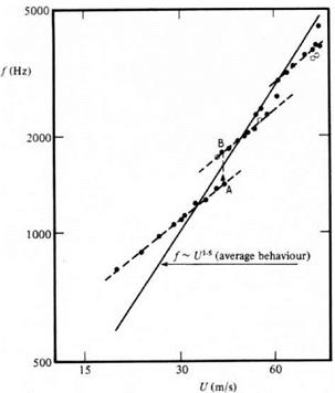 certain integral wave number requirements. The ladder structure is a consequence of a change in the quantization number of the feedback loop. At certain flow velocities, two tones were measured simultaneously. As velocity increases, the dominant tone frequency jumps to the next ladder step as indicated by A to B in Figure 15.20. This is usually referred to as staging. Further velocity increase causes the subdominant tone to vanish. By carefully analyzing their data, Paterson et al. found that the dominant tone followed a U15 power law (see Figure 15.20) where U is the free stream velocity. Based on their extensive measurements, they proposed the following formula for the dominant frequency, f:
![]() 0.011U15
0.011U15
1
(vC)2
where C is the chord width and v is the kinematic viscosity. Eq. (15.41) is referred to as the Paterson formula.
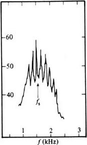
Arbey and Bataille (1983) repeated the airfoil experiment in an open wind tunnel as Paterson et al. did. In all their experiments, the airfoil was at a zero degree angle of attack. Just as Paterson et al. they observed tones. In fact, there is a multitude of them. Figure 15.21 shows a typical spectrum of their measurements. The tones are separated by about 110 Hz. Arbey and Bataille discovered that the frequency of the dominant tone (fs in the center of the spectrum of Figure 15.21) was in good agreement with the Paterson formula (see Figure 15.22). However, there are distinct differences between the two experiments. First of all, Arbey and Bataille measured many tones, but Paterson et al. had at most two tones simultaneously. Moreover, the frequencies of the two tones in the Paterson et al. experiment are separated by a
Figure 15.21. The spectrum of airfoil tones measured by Arbey and Bataille.
 magnitude of about five times that of the tones of Arbey and Bataille. When plotted in a frequency versus velocity diagram, the tones of Arbey and Bataille also form a ladder structure suggesting again that the tones are related to a feedback loop.
Unlike Paterson et al. and Arbey and Bataille, Nash, Lowson, and McAlpine (1999) performed their airfoil experiment inside a wind tunnel. They quickly realized that the cross-duct modes and the Parker modes of the wind tunnel could interfere with the airfoil tone phenomenon. To eliminate this possibility, they lined the wind
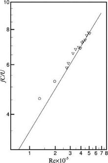 Figure 15.22. Strouhal number of dominant airfoil tone versus Reynolds number measured by Arbey and Bataille. Straight line is the Paterson formula.
|
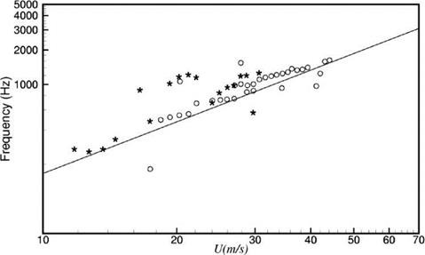
Figure 15.23. Airfoil tones measured by Nash et al. Straight line is the Paterson formula. |
tunnel walls with sound-absorbing materials. Under such an experimental condition, they found that, for each free stream velocity, there was a single tone and no ladder structure. They suggested that the ladder structure data of Paterson et al. and Arbey and Bataille were influenced by their experimental facilities. The feedback and ladder structure of the data were not characteristics of the airfoil tone phenomenon. The feedback loop apparently was locked on something in the experimental facility outside the open wind tunnel. At a low angle of attack, the tone frequency-flow velocity relation measured by Nash et al. is also in good agreement with the Paterson formula (see Figure 15.23). At a high angle of attack, because of the blockage of the wind tunnel by the model, the measured relationship deviates from the Paterson formula, as would be expected.
It should be clear at this time that there is little agreement among the most prominent airfoil experiments reported in the literature. One major issue is whether the basic tone generation mechanism is related to a feedback loop, which would generate multiple tones or, as in the observations of Nash et al., feedback is spurious and there should only be a single tone. Even among investigators who observed multiple feedback tones, the details of the observed phenomenon are quite different. Therefore, it is fair to say that, up to the present time, no two experiments have the same results. The only agreement of all the major experiments is that the Paterson formula is a good prediction formula for the dominant tone frequency. This is true over a wide range of Reynolds numbers.
One way to resolve the disagreement is to perform highly accurate numerical simulations of the phenomenon. Numerical simulation has a number of advantages. First of all, when properly carried out, it can avoid facility-related feedback. Another advantage is that there is no background wind tunnel noise inherent in an experiment. It is no exaggeration to say that numerical simulation is, perhaps, the simplest way to reproduce the tones of a truly isolated airfoil. Finally, numerical simulation provides
a full set of space-time data of the flow and acoustic fields that would facilitate the investigation of the tone generation mechanisms.
Eq. (15.17) gives a direct mapping of the airfoil from the physical plane to the w plane. After the computation, it will be necessary to reverse the procedure to find the point z corresponding to a point w in the transformed plane. For the mapping function under consideration, it is easy to see that away from the airfoil z = w – iQ. Therefore, for these points, the inverse mapping may be found by simple Newton iteration.
Let zn +1 = zn + Azn be the point in the z plane corresponding to the point w = w0 in the w plane after the (n + 1)th iteration. Eq. (15.17) gives
By expanding the terms on the right side of Eq. (15.24) for small Azn, and ignoring all higher-order terms, it is straightforward to find that
To start the iteration, the obvious choice is to take z1 = w0 – iQ.
For points closer to the airfoil, it is advantageous to keep the second-order terms in expanding the right side of Eq. (15.24). Let
(15.27)
where 7 = d/dZ.
Points on the slit in the w plane are more difficult to invert. To invert these points, the following numerical method may be used. Let ws be the point of which the inverse, say zs, is to be found. Suppose the inverse of a point w denoted by z near ws is already found. w may or may not be on the slit. Let w be a point on the line joining w to ws so that
![]()
w — w = reie.
Now, by Eq. (15.17) it is readily found that
On combining Eqs. (15.28) and (15.29), along the line joining w and ws, the following differential equation is established:
zs may now be determined by integrating Eq. (15.30) from r = 0to r = |ws – w| with starting condition r = 0, z = z.
The importance of having a well-designed grid in a numerical simulation cannot be overemphasized. For problems involving solid surfaces, a body-fitted grid is most desirable. Computation on such a grid has the advantage that the wall boundary conditions can be enforced with relative ease and accuracy. With body-fitted grid, one set of grid lines will be parallel to the solid surface. This is ideal for computing the boundary layer adjacent to the wall. Developing a body-fitted grid is not straightforward. Grid generation is, by itself, a topic that has been extensively researched. The subject matter is treated in specialized books and advanced texts. It is beyond the scope of this book to treat grid generation other than providing an example to illustrate some aspects of the basic ideas.
15.3.1 Conformal Transformation
Consider the problem of computing the flow around a two-dimensional airfoil. A simple way to generate a body-fitted grid for the airfoil is to use the method of conformal mapping.
Figure 15.15. Mapping of an airfoil into a slit by conformal mapping. Open circles are sources points on the camber line. Black circles are enforcement points.
![]() The method consists of two essential steps as schematically illustrated in Figures 15.15, 15.16, and 15.17. The first step is a mapping of the airfoil in the physical x – y plane into a slit in the w or the f – n plane. This is accomplished by conformal transformation using a multitude of point sources or doublets distributed along the camber line of the airfoil as shown in Figure 15.15. If point sources are used, the appropriate form of the conformal transformation is
The method consists of two essential steps as schematically illustrated in Figures 15.15, 15.16, and 15.17. The first step is a mapping of the airfoil in the physical x – y plane into a slit in the w or the f – n plane. This is accomplished by conformal transformation using a multitude of point sources or doublets distributed along the camber line of the airfoil as shown in Figure 15.15. If point sources are used, the appropriate form of the conformal transformation is
w = z + £ Qj log Z—j + in, (15.17)
j=1 z z0
where w = f + in is the complex coordinates of a point in the mapped plane, z = x + iy is a point in the physical plane, Qj, Zj (j = 1,2,…, N) are the source strengths and locations, and П is just a constant. The inclusion of П in the mapping function is important. Its inclusion makes it possible to map the airfoil onto a slit on the real axis of the w plane (see Figure 15.16). z0 is the location of a reference source. A good location to place z0 is in the middle of the camber line, such that all the lines joining zj to z0 lie within the airfoil. In this way, the branch cuts associated with the log functions of Eq. (15.17) would not present a problem in the computation.
In implementing the mapping, the coordinates Zj (j = 1,2,3,…, N) of the source points are first assigned. A useful rule in assigning the source locations is that the distance |Zj – Zj_x| should be in some way proportional to the local thickness of the airfoil. That is to say, the sources should be closer together at where the airfoil is thin. Now the source strengths Qj (j = 1,2,…, N) are to be chosen to accomplish the mapping. For this purpose, a set of points, zk (k = 1,2,…, M), well distributed around the surface of the airfoil is chosen to enforce the mapping (see Figure 15.15). zk are the enforcement points, and M should be much larger than N. On imposing the conditions that the surface of the airfoil be mapped onto a slit on the real axis of
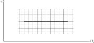 Figure 15.16. Complex w plane. The slit is the airfoil.
 |
the w plane, Eq. (15.17) leads to the following system of linear equations for Qj and ft:
This system of equations may be written in a matrix form (real variable) as follows:
![]() Ax = b,
Ax = b,
where x is a column vector of length (2N + 1). The elements of x are
X2j—1 = Re (Qj), X2j = Im(Qj), j = 1, 2,…, N
X2N+1 = ft.
A is a M x (2N + 1) matrix. The elements of A are
Г zi — zi"
ai,2 j + iai,2 j—1 = log
zi z0
ai,2N+1 = 1’i = 1, 2, . . . , M; j = 1, 2, 3, . . . , N.
b is a column vector of length M. The elements of b are
bk = —yk, k = 1, 2, 3,…, M.
With M > 2N + 1 Eq. (15.19) is an overdetermined system. A least squares solution may be obtained by first premultiplying Eq. (15.19) by the transpose of A. This leads to the normal equation,
ATAx = ATb, (15.20)
which can be easily solved by any standard matrix solver.
If a point dipole distribution is used to map an airfoil into a slit instead of point sources, the mapping function would be
The mapping constants zj, Aj(j = 1, 2,…) and C are determined in the same way as those for point sources.
![]()
The second step in developing a body-fitted grid to the airfoil is to take the midpoint of the slit in the f – n plane as the center of an elliptic coordinate system. The two end points of the slit are the singular points of the conformal transformation. They are given by
![]() dw = 0.
dw = 0.
dz
Let the width of the slit be a and f be the x coordinate measured from the midpoint of the slit. The elliptic coordinates (д, в) are related to (f, n) by
f = 2 cosh д cos в, n = a sinh д sin в. (15.23)
The elliptic coordinate system is shown in Figure 15.17. The elliptic coordinate system is orthogonal. The curve д = 0 is the surface of the airfoil in the physical plane. If the computation is for a flow past the airfoil, then the boundary layer lies in the region д < A in the д – в plane. The wake is in the region – A1 < в < Д2, where A, A1; and Д2 are small quantities for a flow fromleft to right. In a simulation, these are the regions where very fine meshes are needed.