Category COMPUTATIONAL AEROACOUSTICS

The first step in performing a computational aeroacoustics (CAA) simulation is to formulate the problem. This means the development of a computational model. Usu­ally this will include the selection of appropriate governing equations and physical boundary conditions.

In most practical CAA problems, the flow involved is turbulent (a discussion of turbulence modeling will be given in Section 15.5). Since direct numerical simulation of turbulent flow is prohibitively expensive in terms of computer resources required, some simplified method to treat the turbulence of the phenomenon is generally adopted. One may use a Reynolds Averaged Navier-Stokes (RANS) approach. The main advantage of using a RANS model is that it is easy to implement and not very expensive. The disadvantage is that it is not very accurate for time-dependent problems. Recently, the use of large eddy simulation (LES) and very large eddy simulation (VLES) has become quite popular. However, there is still a debate on how to close the LES model. One way is to use a subgrid scale model. The intent of a subgrid scale model is to model the effects of the spectrum of unresolved wave number on the resolved wave number spectrum of the computation, but it has been found that a subgrid scale model often performs only as a dissipation mechanism for the small-scale turbulence in the computation. For this reason, many investigators choose an alternative way. The alternative way is to use artificial numerical damping to remove the very small scale turbulent motion from the computation to avoid accumulation of energy in this wave number range (note: energy is cascaded up the wave number space to the highest wave number range supported by the compu­tation). Excess energy accumulation in the smallest scales could cause a numerical simulation to blow up.

In many CAA problems, viscous effect is important only in a part of the com­putation domain. This may be because of a change in the dominant physics of the phenomenon in different parts of the computation domain. For example, near a wall, the viscous effect is important, while away from the wall, the compressibility effect may be most important. In such cases, the computation model will consist of the use of the Navier-Stokes equation in a part of the computation domain and the Euler equations in the remaining region.

Because a computational domain is finite, the influence of the flow and acoustic fields or sources outside may not be negligible. In such cases, the boundary conditions are forced to reproduce the outside influence as precisely as possible. In such a situation, the boundary condition is a crucial part of the computational model.

The objective of this chapter is to discuss how to design a computation code to simulate an aeroacoustic phenomenon. In previous chapters, many methods and elements of numerical computation were discussed. In this chapter, they are to be synthesized to form a computer simulation code. The basic elements/ingredients of a good simulation algorithm in computational aeroacoustics would consist of the following:

1. A computational model containing all essential physics of the aeroacoustic phe­nomenon

2. A properly chosen computational domain

3. A well-designed computational grid

4. A least dispersive and dissipative high-resolution time marching algorithm

5. A time step that ensures numerical stability and good resolution

6. A set of high-quality boundary conditions for both exterior and interior bound­aries

7. A properly chosen distribution of artificial selective damping to suppress the generation and propagation of spurious short waves

8. A set of properly prescribed initial conditions

15.1 Basic Elements of a CAA Code

Each of the eight elements in this list affects the simulation in some way. Some exert an influence on numerical stability. Some affect the accuracy and quality of the computed solution. Others control and influence the computation time. A more detailed consideration of some of these elements in this list is provided next.

To provide a simple validation test for formula (14.102), reconsider the case of the monopole noise source problem discussed in section 14.5.2 (see Figure 14.12). Instead of a time periodic source, it is replaced by the broadband monopole source of Section 14.6. The half-apex angle of the conical surface 5 is again taken to be 10°. In this case, if Yr is a point on the conical surface, then

Y’ = (R’2 + x2 – 2R’xc cos 5)2.

The two-point space-time correlation function has the following form (see Eq. (14.91)):

Ф(ІЇ, R", &,X) = F

The F-function as computed directly is shown in Figure 14.19. In this special case, Ф is independent of ©. For this reason, the integral over d& in Eq. (14.102) is zero except for n = 0. Thus the far-field noise spectrum obtained by continuation of the pressure field on the conical surface is as follows: [16]

A change of integration variable from X to n = (Y" – Yr – a0X)/D transforms the triple integrals in Eq. (14.103) into three separate integrals. This yields

s (Яв, ф,ю) D

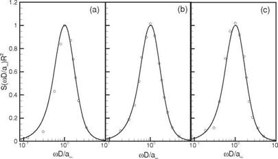
Figure 14.21 shows a comparison of the far-field noise spectra at в = 150°, 90°, and 30° (exhaust angle) computed numerically according to Eq. (14.104) and the original noise spectrum of the broadband monopole source (the similarity spectrum of the noise of large turbulence structures of high-speed jets). The agreement is excellent. The excellent agreement provides strong support for the validity of the present continuation method.

EXERCISE

An important CAA problem is to compute the noise of a high-speed turbulent jet. Since a computational domain is finite, it extends only to the near acoustic field. To determine the far-field sound, the continuation method developed in the Section

14.6 may now be used. The noise of a turbulent jet is broadband and random. It contains an enormous amount of information. However, for practical purposes, the

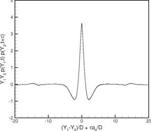
Figure 14.19. The two-point space-time correlation function computed accord­ing to Eq. (14.92).

quantities of interest in the far field are the noise spectra and directivity. For this reason, only the continuation of the noise spectra from the near field to the far field at different angular direction is considered.

In Section 14.5, it was suggested that a good choice of a matching surface Г is a conical surface as shown in Figure 14.8. A method to compute the surface Green’s function p(g) (R, в, ф, t; R0, ф0, t0) through the use of the adjoint Green’s function has also been developed. Let ps(R0, ф0, t0) be the pressure of a turbulent jet measured on the conical surface. The conical surface has a half-apex angle of 5. The far-field pressure is then given by

p(R, в, ф, t)

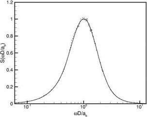Figure 14.20. Comparison between the original (full line) and the computed spectrum (dotted line). The computed spectrum is the Fourier transform of the correlation function F (-f ) given in Figure 14.19.

By Eq. (14.75), the Fourier transform of the surface Green’s function may be expanded in a Fourier series in (ф — ф0), that is,

Now, the far-field noise spectrum, S(R, в, ф, ю), is the Fourier transform of the autocorrelation function, i. e.,

In Eq. (14.95), the angular brackets, {), are the ensemble average of the random variables inside the brackets. Since the sound field is stationary random, the ensemble average and the time average are equal. By means of Eqs. (14.93) to (14.95), the following relation between the spectrum function and the source function can easily be established.

TO TO

E E {ps (R’,ф, t’)ps (r"a" , t"))

m=—to п=—то

x pm (R, в; R’, ю’)pn (R, в; R", ю" )

~—ію'(ї —V )—ію/'(ї—Ґ’)+іт(ф—ф/)+іп(ф—ф/’)—ію/’т+іют x e

x R R’ sin2 SdrdoJdoJ ‘ dt’ dt” dR dR’ dф’ dф”. (14.96)

For jet noise, the surface pressure ps is a stochastic variable that is stationary random in time and homogeneous in the azimuthal variable ф. These properties allow the two-point space-time correlation function to be written as

{ps(R, ф’, t’)ps(R, ф”, t")) = <b(R, R", ф’ — ф”, t’ — t"). (14.97)

On inserting Eq. (14.97) into Eq. (14.96), the far-field spectrum function becomes

2?//f"f £ £ фr —ф"’•’—

J J J J m=—to n=—to

x pm (R, в; R’,ю’)pn (R, в; R ‘,ю")

X е~ію’ (t— ) —ію” (t—t’ )+m (ф—ф1) +іп (ф—ф")—ію"т +іют

X R’R" sin2 Sdr dm dm’ dt’dt" dR’dR" dф’d^’. (14.98)

In the following, it will be shown that, regardless of what the two-point space­time correlation function Ф (R, R", ф’ — ф”, t’ — t”) is, five of the integral and one summation in Eq. (14.98) can be evaluated.

The dr integral may be evaluated in a straightforward manner as follows:

TO

The dt’ and dt" integrals may be evaluated by a change of variables to X = t’ -1", f = t". This gives

TO TO

j j Ф(ІЇ, R" , ф’ – Ф", t’ -1”)e-iot-io’fdt’ dt"

TOTO

= j j Ф(R/, R”,ф’ – ^’,X)e-io X-i(o +o")f df dX

-TO – TO

TO

= 2n5(o’ + o”) j Ф(R/, R",ф’ – ф” ,X)e-io X dX. (14.100)

The d^ and dф" integrals may also be evaluated by a change of variables to

© = ф’ – ф” and Ф = ф”, thus,

2n 2n

j j Ф(ІЇ, R", ©,Х)е-ітф-іпф’d^dф”

00

2n 2n

= j j Ф(R/, R",©,X)e-im©+i(m+n)’l‘dVd©

00

2n

= 2n5m,-n / Ф(ІЇ, R", ©, X)e-im©d©. (14.101)

0

Substitution of Eqs. (14.99) to (14.101) into Eq. (14.98), and upon integrating over do’ and do” and summing over m, the mathematical formula for the noise spectrum is

S(R, в, ф, о)

to to 2n to to

= 4n2ffff ^2 Ф(^, R, ©, X)P-n(R, e; R, – o)pn(R, e; R",o)

0 0 0 – TO n=-TO

x eioX+in©R’R" sin2 5 dXd©dR’dR". (14.102)

Eq. (14.102) is the principal result of this section. Physically, it signifies that the two-point space-time correlation function is the equivalent noise source on the conical surface. If this function is known, either by experimental measurement or by numerical simulation, then the far-field noise spectrum can be computed. Note: the dX and d© integration apply only to the equivalent noise source function. These two operations effectively decompose the source into frequency and azimuthal components.

Eq. (14.102) has been used in the experimental work of Tam, Viswanathan and Pastouchenko (2010) (see also Tam, Pastouchenko and Viswanathan (2010)). They measured the near-field two-point space-time pressure correlation function Ф(№, R", ©, X) of a Mach 1.66 hot jet on a conical surface of 100 half-angle. They
used Eq. (14.102) to determine the far-field noise spectra. They showed that the noise spectra continued from the near-field were in good agreement with the measured far-field spectra.

Many aeroacoustics problems involve noise generated by turbulence. For this class of problems, both the source and the sound field are random and consist of a broad spectrum of frequencies. This is the case of high-speed jet noise. At a high Reynolds number, the jet flow is turbulent with a wide range of length scales. The noise emitted is broadband typically spread over three decades of frequencies. At the present time, there are not enough computational resources to perform direct numerical simulations of the jet flow. Many investigators choose to use large eddy simulation (LES) as an alternative, but the computational domain is finite and often is minimized to reduce computational cost. For this reason, without exception, only the acoustic near field is computed. However, for community noise purposes, interest is in the far field. Therefore, a method capable of continuing broadband near acoustic field to the far field is very much needed.

In Appendix F, a method to produce real-time pressure waves from a random broadband noise source is described. For a broadband monopole source, the acoustic field generated is spherically symmetric. Consider such a localized source as shown in Figure 14.12. Suppose the noise spectrum S(s-D) is given where D is the length scale and a0 is the speed of sound. The sound field emitted by the monopole source following Appendix F is as follows:

(Ю

p(Y, t) = — A(m) cos

Figure 14.16. The similarity spectrum of the noise of large turbulence structures of high-speed jets. This spectrum is used as the noise spectrum of a broadband monopole source measured at Y/D = 1.0.
On following the energy-conserving discretization procedure, the discretized form of this equation is (see Eq. (F9)) as follows:
rnD a0
2S	(14.90)
p(Y, t)
j
j
a0
As a numerical example, suppose the noise spectrum S(sD) has the same shape as the similarity spectrum of the noise from the large turbulence structures of high­speed jets (see Tam, Golebiowski, and Seiner (1996); Tam, Viswanathan, Ahuja, and Panda (2008)). The similarity spectrum is shown in Figure 14.16. Note: the spectrum is assumed to be symmetric, i. e., S(-^) = S(^D). Upon dividing the spectrum into 250 bands, the spatial distribution of pressure in the wave field at a selected instant of time, according to Eq. (14.90), is shown in Figure 14.17. Figure 14.18 shows the time history of pressure fluctuations measured at a distance of Y = 5D from the monopole source. The random fluctuations are time stationary, that is, the stochastic properties of the broadband sound field is independent of time. An arbitrary starting time is used for the display in Figure 14.18.
Y/D
Figure 14.17. Spatial distribution of the pressure field of a broadband monopole source with a spectrum given by the sim­ilarity spectrum of Figure 14.16.

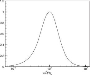
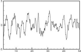
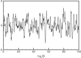
Figure 14.18. Time history of pressure fluctuations at Y = 5D from the broad­band monopole noise source of Figure 14.17.

The two-point space-time correlation function of the broadband sound field of a monopole source, following Eq. (F5), is given by

where the overbar means the time average. The function F(Y2 YD a°) can also be computed directly from the acoustic field of the monopole source, that is,

Y — Y —a t

Figure 14.19 shows the two-point space-time correlation function F ( 2 d 0 ) as computed directly according to Eq. (14.92). As a check on the accuracy of the energy – conserving discretization method and this formulation, the noise spectrum S(^D) is calculated by taking the Fourier transform of F(D), obtained by setting Y1 = Y2. This should yield the original prescribed similarity spectrum. A comparison of the two spectra is given in Figure 14.20. This figure indicates that there is good agreement between the two spectra. This confirms that the energy-conserving discretization method can, indeed, generate a broadband sound field with a given spectrum.

For time periodic sources with time dependence e—iQt, the source function on the conical surface may be written in the following general form:

в = 5, psource(R, Ф0, t0) = *(R>. Ф0)e—iQt0. (14.82)

By Eq. (14.61), the far-field pressure field (R ^ ж) associated with the source is given by

p(g)(R, в, ф; R0, ф0; m, t0)^(R0, ф0)e~imt—iQt°R0 sin 5dm dt0dR0 dф0.

(14.83)

On using p(g) in a Fourier expansion in (ф — ф0), i. e., Eq. (14.75), Eq. (14.83) becomes after integrating over dt0 (giving rise to 2п5(ш — О)) and then upon inte­grating over dm,

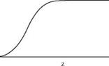Figure 14.11. A typical profile of damping function a(z).

Y

2npm(R, в; R0, n^(R0, ф0)еіт(ф-ф°)-tatR0sinSdR0 йф0,

0 0

(14.84)

where pm (R, в; R0, a) is given by Eq. (14.76). In this form, only two integrations need be evaluated.

As a concrete example, consider a time periodic monopole source located at a distance xc from the apex of a conical surface as shown in Figure 14.12. Let Y be the distance of a point from the monopole source. For a point on the conical surface with a spherical polar coordinates (R0, 5, ф0), Y for this point is given by

Y0 = R0 + x2 – 2R0xc cos 5)2. (14.85)

The pressure field on the conical surface associated with the monopole acoustic source is

Thus, in the notation of Eq. (14.82), the Ф function is

e‘QY0/a0

4nY0

Substitution into Eq. (14.84), the far pressure field of the monopole source, according to the continuation method, is as follows:

In deriving Eq. (14.88), the integral over ф0 has been performed. This integral is zero except for m = 0. Note that p0 is given by Eq. (14.76). The remaining integral

Figure 14.13. Computational domain for the monopole acoustic source.

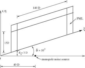
over R0 has to be evaluated numerically. The first step is to compute the adjoint Green’s function v0a) and іл^ in the f – n plane as discussed before. These two quantities are required to compute p0. For the present example, a computational domain with a size as shown in Figure 14.13 is used. The half-apex angle 5 is 10°. Note that a conical surface has no intrinsic length scale. Here, D in Figure 14.13 is taken as the length scale. In the far field, R ^ ж, the directivity factor is defined by

where p is given by Eq. (14.88). For ^ = 1.0, the computed results are shown in

ao

Figures 14.14 and 14.15 for a source located at xc/D = 40.0. The exact solution

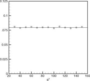Figure 14.14. The computed directivity of a periodic monopole. The straight line is the exact solution.

Figure 14.15. The computed phase of an off-center periodic monopole. Full line is the exact solution.

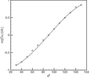_ a D(в, Or)

is D(e ) = |D (в, )| = 4L and arg[ ] = – cos в. The phase factor arises

because the source is not located at the origin of the spherical polar coordinate system. As can be seen, the agreements between the magnitude and phase of the computed results and the exact solution are good. This provides confidence in the numerical method.

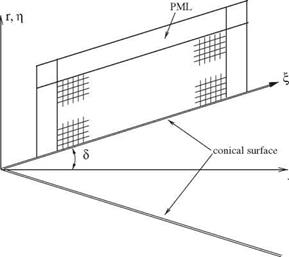
A relatively simple way to compute the homogenous solution is to convert Eqs. (14.66) to (14.69) into time-dependent equations by replacing – io by Jt and add a factor of e-imt to the right side of boundary condition (14.70). The resulting problem may then be time marched to a periodic state, which is the nonhomoge­neous adjoint solution. For this purpose, it is advantageous to switch to an oblique Cartesian coordinate system (f, n) as shown in Figure 14.9. The oblique Cartesian coordinates and the cylindrical coordinates are related by

x

n = r – x tan S, f = or r = n + f sin S, x = f cos S. (14.78)

cos S

With respect to the oblique Cartesian coordinates, the adjoint equations (14.66) to (14.69) in the time domain may be rewritten in the following form:

where

‘ u(a) ‘ um vm

«0 sec 8 0 0 0

/ 0 0 0 0 0 0 0 0 0 – sec8 0 0

„-i—t

A

The boundary condition on the conical surface is

ц = 0, pm = – j( —f sin вх sin 8 ) e-i—(fcos 5 cos 0i+t). (14.80)

a0 /

To avoid the reflection of outgoing disturbances back into the computational domain, it is recommended to install a perfectly matched layer (PML) around the computational domain as shown in Figure 14.9. It is straightforward to develop a set of PML equations. A split-variable version of these equations is

In Eq. (14.81), a is the damping function. Figure 14.10 shows a distribution of a(z) in the f – ц plane. For best results, it is recommended that a profile of a(z) resembling that in Figure 14.11 be used.

The solution of Eq. (14.79) together with PML boundary condition (14.81) and nonhomogeneous boundary condition (14.80) may be computed by using the 7-point stencil dispersion-relation-preserving (DRP) scheme. Boundary condition (14.80) may be enforced by the ghost point method. This boundary condition is responsible for introducing the correct disturbances into the computational domain. Since a time periodic solution is sought, a zero initial condition is the simplest way to get the solution started. The solution is to be marched in time until a time periodic solution is reached. Note: the adjoint Green’s function is spatially oscillatory because boundary condition (14.80) is an oscillatory function. The period of oscillation of boundary condition (14.80) may be used to estimate the spatial resolution required for computing the adjoint Green’s function. Experience suggests that it is prudent to turn the nonhomogeneous boundary term on gradually. This may be done by multiplying the right side of boundary condition (14.80) by a factor (1 – e^t/T) and taking T to be a number of oscillatory periods long. The reason for this is that, after discretization, the response of the finite difference system to a sudden imposition of boundary condition is sometimes not the same as that for a partial differential system.

The noise of high-speed jets is an important aeroacoustic problem. Because the mixing of the jet and ambient gases, the jet expands laterally in the downstream direction. The use of a cylindrical surface Г for this type of flows would not be appropriate. A conical surface with a well-chosen half-angle 5 is a good choice. Figure 14.8 shows a conical surface Г enclosing a high-speed spreading jet. The natural coordinates to use outside the conical surface is the spherical polar coordinates (R,0,Ф).

Let p(g)(R,0,ф, t; R0^0, t0) be the direct surface Green’s function with the source point located at (R0, ф0) and source time t0. The Fourier transform of time t is

(14.60)

The far-field sound pressure due to a surface pressure distribution of Ф (R0, ф0, t0) on the conical surface is then given by

p(R, 0, ф, t) =

to 2n to to

//// pig)(R, 0, ф; R0, ф0; o; Ц)Ф^0, ф0, t0)e

—TO 0 0 —TO

The surface element of a conical surface is dS = R sin SdRd(p. By the reciprocity relation of Eq. (14.52), p(g) is related to the adjoint Green’s function v’f’1 by

p®(R1> $1, ф1; R0, ф0; t0) = v^ (R0, ф0; R1, в1, ф1; to), (14.62)

where v(n) is the adjoint velocity component normal to the conical surface Г. Positive is in the outward pointing direction.

As for the case of a cylindrical surface, a particular solution of the adjoint equations is given by Eq. (14.55). The relationship between cylindrical coordinates and spherical coordinates is

r = R sin в, x = R cos в.

On replacing r and x by this relation and upon using Eq. (14.55), the particular solution (denoted by a subscript “p”) may be written as

СО / ч

p(a) = -2 Д (R1-R cos в cos e1 Jm 2R sin в sin в1 e-im 2 +іт(ф1-ф).

Pp 8n2fl0R1 m=—О ma0 V

(14.63)

The adjoint velocity is related to the pressure by Eq. (14.49). Thus, the compo­nent normal to and on the conical surface is

Now, let the homogeneous solution (denoted by a subscript “h”) of Eq. (14.49) and (14.50) in cylindrical coordinates to have the following form:

This is a Fourier series expansion in angular variable (ф — ф1). The governing equations for the amplitude functions (u(m, vJ, wJ, pm ) can readily be found by substituting Eq. (14.65) into Eqs. (14.49) and (14.50) with the nonhomogeneous term omitted. These equations are as follows:

The boundary condition from Eq. (14.51) is

0 = 5, pm = – Jm[ —R sin 5 sin 01 ) e

a0

For future reference, it is easy to show that by taking the complex conjugate of Eq. (14.66) to Eq. (14.70) that

u—m (r, x; 01, —ю) = am* (r, x; 01, ю) (14.71)

v(—m (r, x; 01, —ю) = v(m’ (r, x; 01, ю), (14.72)

where * denotes the complex conjugate.

Once u(m) and v(m) are found, it is straightforward to find, by combining with par­ticular solution Eq. (14.64), that the normal velocity of the adjoint Green’s function on conical surface 0 = 5 with (R, ф) replacing by (R0, 00) is

mm (R0, ф0; R1, 01, ф1; ^0,ы)

. I UJ

+ i cos 01 sin 5Jm I —R0 sin 01 sin 5

a0

— i [v(m)(R0, 5; ю) cos 5 — , 5; ю) sin 5]} ■ e—imп +т(ф1— ф0). (14.73)

By means of the reciprocity relation (14.62), the pressure associated with the direct Green’s function is now known, i. e.,

For later application, it is useful to expand p(g) as a Fourier series in (ф — ф0) in the following form:

Figure 14.9. An oblique Cartesian coor­dinate system for computing the homo­geneous adjoint Green’s function.

By means of Eqs. (14.74) and (14.73), it is easy to find that

+ i cos в sin SJm sin в sin SR0 e a" 0

a0

v-)(R0S, o) cos S – ui‘ma)(R0tS, o) sin sJJ. (14.76)

% R

Note: The dependence of pm on R is in the factor. An important property of pm (R, в; R0, o) is that it becomes its complex conjugate if m ^ -m and о ^ – o, i. e.,

p-m (Яв; R0> -0) = Pm (R^; R0,o>.

Eq. (14.55) may be regarded as a particular solution of Eq. (14.53). There is also a homogeneous solution. When combining the particular and the homogeneous solution, the full solution satisfies boundary condition (14.51) on the cylindrical surface at r = D/2. In cylindrical coordinates, the appropriate homogeneous solution (denoted by a subscript “h”) is

(14.56)

where Cm is a set of unknown constants. H,(1) () is the mth order Hankel function of the first kind. By adding Eqs. (14.55) and (14.56), the adjoint Green’s function is

. i — (R —x cos 0 )+ШТ

= —Ше a° і 1 8n 2a0>R1

Upon imposing boundary condition (14.51), it is found that

Jm (a;sin 01 z)

»*{ a; si" 01D)

Thus, the adjoint Green’s function p(a) and the radial velocity v(a) are

j~(t0 sin 0‘r) sin 01D)—sin D)sin 0-r

x cos[m^ — ф1)].

On the cylindrical surface, the terms inside the square bracket of Eq. (14.58) may be simplified by using the Wronskian relationship of Bessel functions. This gives

v(я) (D, x, ф; R1? 0Ь ф1; o, т)

By means of the reciprocity relation (14.52), the Fourier transform of the pres­sure of the surface Green’s function is given by the right-hand side of this equation. This expression may be further simplified by noting that

Therefore, by inverting the Fourier transform, the surface Green’s function becomes

p{g) ^,в, ф, t; D, Хо, Фо, т)

Eq. (14.59) is the same as the direct Green’s function of Eq. (14.18).

By eliminating v(a) from Eqs. (14.49) and (14.50), the governing equation for p(a) is found to be

Let (Я, в,ф) be the coordinates of a spherical polar coordinates system with the x-axis as the polar axis (see Figure 14.4). Also, let (r, ф, x) be the coordinates of a cylindrical coordinate system with the x-axis as its axis. For convenience, the source vector x1 is taken to lie on the plane ф = ф1, then

x1 = R1 cos 01ex + R1 sin в1 cos ф1ёv + R1 sin в1 sin ф1ё z. Also, the position vector x is

x = x ёх + r cos ф ё v + r sin ф ё_.

For large R1 (R1 ^ to), the distance between x1 and x is |x ■ x1|

|x1l

Thus, Eq. (14.54) may be rewritten as

where e0 = 1, em = 2 for m > 1. The first line of Eq. (14.55) is just the plane wave solution for a source at a great distance. This is illustrated in Figure 14.7. The second line of Eq. (14.55) is the cylindrical wave expansion (see chapter IX of Magnus and Oberhettinger, 1949). Eq. (14.55) is only a part of the adjoint Green’s function. The second part is the scattered wave. It will be shown that the scattered wave part of the adjoint Green’s function may be computed as a two-dimensional problem.