Category FLIGHT MECHANICS MODELING and ANALYSIS

Aircraft parameter estimation

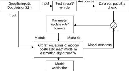
One important aspect of flight-testing of any aircraft or helicopter (or even a missile) is to generate the data for estimation of its stability and control derivatives. In this sense, parameter estimation is an important tool for flight test engineers and data analysts to determine the aerodynamic characteristics of new and untested aircraft. Flight-estimated derivatives are very useful in updating the flight simulator models (of aircraft), improving the flight control laws, and evaluating handling qualities. In addition, flight-determined derivatives (FDDs) help in the validation of the predicted derivatives, which are based on one or more of the following: (1) wind-tunnel experiments on scaled models of aircraft and subsequent data reduction methods; (2) DATCOM (Data Compendium) methods; and (3) some analytical/CFD methods. The aircraft dynamics are modeled by a set of differential equations. The external forces and moments acting on the aircraft are described in terms of aircraft stability and control derivatives, which are treated as unknown parameters. Responses of the test aircraft and the mathematical model are obtained and compared using specifically designed control inputs. An appropriate parameter – estimation algorithm is applied to minimize the error (in responses) by iteratively adjusting the model parameters. The key elements—maneuvers, measurements, methods, and models—play an important role in aircraft parameter estimation (Figure 9.1). Assume that a set of measured flight test time histories are given; the parameter-estimation problem is thus to determine the values of a given set of parameters in the system equations (postulated model), which will provide the best match of the model responses to actual aircraft responses, in either LS or minimum mean square error sense. There are several methods for the estimation of aircraft parameters and the basic differences are due to certain assumptions, choice of optimal criteria, formulation of cost function that reflects the existence of external disturbances, and the presence of measurement noise in the data.

9.3.1 Maneuvers, Measurements, and Mathematical Models

A detailed description of maneuvers that are to be performed specifically for generating data that are suitable for aircraft parameter estimation was presented in Chapter 7. The first major step in aircraft parameter estimation is the definition and planning of flight test experiment and subsequent data acquisition. This primarily addresses the issue of specification of flight test maneuvers and obtaining measure­ments of control surface deflections, airspeed, sideslip, angle of attack (AOA), angular velocities, linear and angular accelerations, and attitude angles. Also, defin­ition of flight conditions, aircraft configuration, sensors, fuel consumption for esti­mation of aircraft, CG location, weight, and inertias is required. Detailed information about these must be sought before the analysis of the flight data.

The accuracy of estimated derivatives depends on the quality of measurements that are subjected to systematic and random errors. It is essential to evaluate the quality of the measured data and rectify these measurements before using them for parameter estimation. These evaluations include consideration of factors like the frequency content of the input signal, sampling rate, signal amplitude, and signal-to – noise ratio. Some quantities may be difficult to measure directly, such as vibration levels in helicopters. As a first step, the raw data is inspected for obvious gross errors and imperfections, such as incorrect signs of measured variables, missing points, spikes, and extensive noise. The corrections are made in data to account for errors resulting from sensor location (e. g., CG offset and flow corrections) and time-skew errors. The procedure for evaluating data quality and correction is the kinematic consistency checking; as the aircraft states are related by a set of differential equations, one checks for consistency among the kinematic quantities. As an example, the measured roll and pitch altitudes should match with those reconstructed from the rate measurements with great accuracy. The process ensures that the data are consistent with the basic underlying kinematic models; since the aircraft is flying, it must be according to the kinematics of the aircraft, but the sensors could have gone wrong in sensing/generating the data. The data compatibility check provides the estimates of the bias parameters and scale factors in the measured data. An accurate determination of these errors is very important for accurate estimation of the aero­dynamic derivatives from flight data.

The mathematical models used in aircraft parameter estimation are discussed in Chapters 3 through 5 and specifically simple longitudinal and lateral-directional (LD) models are discussed in Chapter 5. If the modes of aircraft dynamics are not properly excited by the chosen input, then an attempt to identify too many para­meters from a limited amount of data might fail or yield estimates with reduced accuracy.

The response of an aircraft to pilot’s (or computer’s) command signal is the flight data that along with other mandatory data (mass, inertia, dynamic pressure, etc.) are used in a parameter-estimation procedure to estimate the aerodynamic derivatives. These responses are generated by exciting certain modes of the aircraft. These modes

are dynamic modes and they contain information on the aerodynamic derivatives implicitly. It is essential to choose input test signals with good characteristics so that properly excited dynamic responses are available for further analysis. The test input signal must possess certain desirable features: (1) it should have sufficient bandwidth to be able to excite the modes of interest; (2) the amplitude and form of the signal should be able to yield good quality maneuver; (3) the amplitude, bandwidth, and slope of the signal should be bounded so that aircraft motion does not violate the assumption of linearity; and (4) the pilot should be able to realize (generate) the signal easily. Of course, for complicated signals computer simulation or prerecording can be used. To design a multistep input signal, which will excite the modes of an aircraft, one can use the Bode diagram approach [13]. This allows one to select the frequencies to be included in the signal based on the identifiability of the derivatives.

Transfer Function Models from Real-Flight Data

It is often advisable to fit a TF to the real flight data to quickly assess the dynamic characteristics of the aircraft. TF and the Bode plots can be easily obtained using the SID toolbox of MATLAB. The main principle is that an output/input mathematical form like the LS model is fitted to the discrete-time data and the Bode diagram from this model is determined [10]. Another approach is to fit a TF model to the frequency response data (the amplitude vs. frequency and the phase vs. frequency data) by the LS method [3]. From this TF again the Bode plot can be obtained. These two approaches are available in the MATLAB toolboxes. Basically, it is a system identification/ parameter-estimation problem and the criterion for the minimization would be the same as in time domain, except that here we are dealing with frequency domain data instead of time histories. One can fit a delta operator TF to the continuous-time data of a dynamic system [11], the merits of which are discussed in Section 2.2.1.

The ‘‘arx’’ model of second order was fitted to the real flight data (of a transport aircraft) using the following sequence in MATLAB:

Data = iddata(q, ele,0.4); model = arx(Data,[2 1 0])

A(q-1) = 1 – 1.981q-1 + 0.9898q-2 B(q-1) = -0.002198

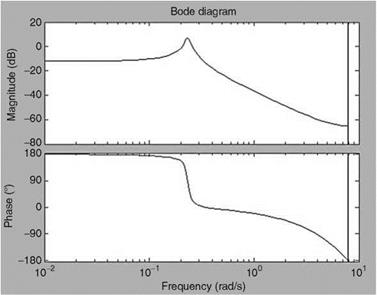
The discrete time Bode diagram was then obtained by dbode([-0.002148], [1 -1.981 0.9898], 0.4). Figure 9.3 shows the Bode diagram of this pitch rate-elevator control input TF.

image178

FIGURE 9.3 Frequency response of the pitch rate to elevator TF estimated from real flight data of a transport aircraft.

9.2.2 Expert Systems for System Identification

Although the SID procedure is well established, there is still some scope for improvement until perfection is achieved. A typical exercise would need a dozen steps. It should be possible to build an expert system that utilizes a set of rules that attempt to mimic the way in which an experienced SID expert proceeds while still using the ID toolbox of MATLAB. The expert system (SIDES) should be able to run without any intervention from an analyst. SIDES would start its iterative journey once driven by the data and rules. SIDES would have the following features: (1) an efficient sampling device with appropriate filters to select the data at lower sampling intervals without loss of information and (2) a set of permissible model structures. A typical expert system has the following steps [12]: (1) parsimonious walk through the model set defined by the analyst; (2) selection of best models based on a quality index; and (3) modification of the sampling interval. The first step avoids the examination and comparison of all the models in the model set. The quality index reflects the best trade-off among many validation tools. The rules are goal oriented and every set of rules is organized around a particular goal. Each rule would contain a conditional expression of one or more patterns, which would be followed by an unconditional action.

Comparison of Several Model Order Criteria

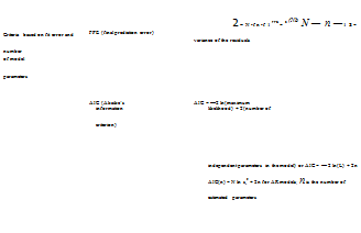
The crucial aspect of time-series modeling is that of selection of model structure (AR, MA, ARMA, or LS) and the number of coefficients for fitting this model to the time-series data. There are several model order selection criteria available in the literature [1,10]. Selection of a reliable and efficient test criterion could be difficult, since most criteria are sensitive to process-statistical properties, which are often unknown. In the absence of a priori knowledge, any system that is generating time-series output data/signals could be represented by the more popular AR or LS model structures. These structures represent a general nth order discrete linear time-invariant system affected by random noise. The problem of model order determination is to assign a model dimension to adequately represent the unknown system, and the model selection procedure involves selecting a model structure and its complexity. Often a model structure can be ascertained based on the knowledge of the physics of the system. For certain processes, if physics is not well understood, then a black-box approach can be used, leading to a trial and error iterative proced­ure. In many situations, some knowledge about the system or the process would be available. Several model selection criteria arising out of different, but sometimes related, principles of goodness of fit and statistical measures are possible. The criteria based on fit error of estimation, number of model parameters/coefficients, and whiteness of residuals are given in Table 9.1.

TABLE 9.1

Comparison of Some Model Order Selection Criteria

Criteria based

FEC1 (fit error

N

1/n£ [zt-zt(ft)]2

If FEC1 < 1 select the model

on the

criterion)

FEC1 =——————- ^————————

with Ьь

concept of

1/n£ [zt-zt(b2)]2

If FEC1 > 1 select the model

fit error

N = number of data

with b>2.

points

FEC2 (fit error

N

1/N^] [zt-zt(b)]2

Insignificant change in the value of

criterion)/PFE

FEC2 =——————————————

FEC2 determines the order of the

(prediction fit error

1/NT.4

model by locating the knee of the

criterion)

curve FEC2 vs. model order.

PFE = FEC2 x 100.

Подпись: Comparison of Some Model Order Selection Criteria
Подпись: RSS (residual sum of squares)
Подпись: With a new parameter in the model there should be large reduction in the RSS. Useful for models of output/input types.

TABLE 9.1 (continued)

Подпись:Подпись:Подпись: DFE = zПодпись:Подпись:Подпись:If the two models are equally likely (L1 ~ L2), then the one with less number of parameters is chosen again according to the principle of parsimony. If the number of parameters increases, the AIC also increases, and hence the model is less preferable.
The test based on whiteness of residuals is widely used to check whether the residuals of fit are a white noise sequence. Autocorrelation based whiteness of residuals (ACWRT) test is performed as shown in Table 9.1. Here, it is assumed that r(k) is a zero mean sequence. Autocorrelations must lie in the band ±1.96 Д/N at least for 95% of the time for the null hypothesis and usually the normalized ratio is used: Rrr(r)/Rrr(0). Autocorrelations tend to be impulse function if the residuals are uncorrelated, and hence at other times their values must be too small, within the above-prescribed bounds. For input/output (I/O) type models (ARMA, transfer function [LS]), the process of cancellation of zeros with poles provides a model with less complexity. The numerator and denominator polynomials are factored and cancellation, if any, then becomes obvious, but a subjective judgment is involved, since the cancellation might not be perfect. Often eigenvalues are used for model reduction and selection. Eigenvalues cannot be meaningfully determined for a covariance matrix if I/O units differ. Dimensional inconsistencies can be removed
by appropriate normalization of the covariance matrices used in the computation of model order criteria.

Detailed modeling using time-series and transfer function analysis is covered in Ref. [10], wherein three applications of model order determination are consid­ered. The data sets were derived from (1) a simulated second-order system, (2) experiments with a human operator in a fixed-base simulator, and (3) forces on a scaled-down model of an aircraft in a wind tunnel exposed to mildly turbulent flows. For the simulated system, AR model identification was carried out using the LS method and it was found that several model order criteria, studied in the foregoing, provided sharp and consistent decisions. Next, the time-series data for the human operator’s responses were derived from a compensatory manual control tracking experiment on a fix-base research flight simulator. Before recording the data the operator was allowed to reach his steady performance in the tracking task. The LS/AR models were fitted to the data and several model order determination criteria were used and studied. Five hundred data points sampled at 50 ms were used for SID. A fifth-/sixth-order AR model for human activity in the tracking task was found suitable, whereas the LS model of second order was found to be also suitable for the same data sets as can be seen from Table 9.2.

From the discrete Bode diagrams obtained for the LS models, it was found that adequate amplitude ratio (plot vs. frequency) was obtained for the second-order TF. Thus, the AR pilot model differs from the LS pilot model in model order because the LS model has distinct I/O structure and hence the data is well captured by the numerator also. This is not so for the AR model and hence a longer (large order) model is required. Estimation of pitch damping derivatives was attempted using random flow fluctuations inherent in the tunnel flow, wherein an aircraft’s scaled physical model was mounted on a single DOF flexure with a dominant second-order response. The excitation to the model was inaccessible and not measurable, being the random flow fluctuation of the tunnel itself. AR models were fitted using 1000 sample data. Since response was known to be of second order, the natural frequency was determined by evaluating the spectra using a frequency transformation of discrete AR models. The estimated natural frequency stabilized for AR(n), n > 10.

Based on the experience gained, using several model order criteria, the following working rule is considered adequate for selection of the model order to fit varieties of experimental data. For order determination: (1) evaluate entropy criterion (AR only), (2) evaluate FPE, (3) perform F-test, and (4) check for pole-zero cancellations (for I/O model). For model validation: (1) see time-history prediction, (2) test residuals for whiteness, and (3) do the cross validation.

TABLE 9.2

Human Operator’s LS Model from the Tracking Experiments

Criterion/Order

n = 1

n = 2

n = 3

n = 4

n = 5

% FEC2

3.13

0.03

0.03

0.046

0.08

% DFE

94.07

17.70

19.17

72.7

System Identification and Parameter Estimation

9.1 INTRODUCTION

The system identification and parameter-estimation process (SIPEP), one of the important approaches to mathematical modeling, provides a powerful tool for sys­tematic analysis and eventual optimization of industrial processes, thereby reducing losses and saving the cost of production. The SIPEP is a fairly mature technology and can be considered as a data-dependent model building process. In aerospace applications it can be used to great advantage to aid the iterative control-law design/flight simulation cycles as well as in certification of atmospheric vehicles. System identification (SID) refers to the determination of an adequate mathematical model structure based on the physics of the problem and analysis of available data using some optimization criterion to minimize the sum of the squares of errors between the responses of the postulated mathematical model and the real system. The computational procedure is generally iterative and requires engineering judg­ment and use of objective model selection criteria [1]. Parameter estimation is also employed in the SID procedure. Parameter estimation is regarded as a special case of SID procedure and also of Kalman filtering methods. Parameter estimation refers to explicit determination of numerical values of unknown parameters of the postulated state-space mathematical model, or any type of the model. The basic principles are the same as in SID but in many cases the model structure selection procedure may not be needed due to the availability and use of well-defined structure from the physics of the system (Chapters 3 through 5), e. g., aircraft parameter estimation. The SIPEP for a flight vehicle is illustrated in Figure 9.1.

The SIPEP utilizes techniques and principles from several established branches of mathematics, science, and engineering: (1) general and applied mathematics for definition of mathematical models; (2) statistical and probability theory for inter­pretation of results and definition of cost functions/criteria (Appendix B, [2]); (3) optimization methods and theory of model reduction for optimal solutions; (4) numerical techniques for solution of differential equations and matrix inversion; (5) system and control theory for state-space and transfer function modeling (Appen­dix C, Chapter 2); (6) signal processing for fast Fourier transform (FFT), spectral density evaluation, and filtering of signals (Appendix C); (7) linear algebra for vector/matrix and related theories (Appendix B); and (8) information theory for interpretation of results and definition of criteria. More often the configuration of the SIPEP used for a particular application is governed by the state-of-the-art

Maneuvers Measurements

image176

FIGURE 9.1 System identification/parameter estimation procedure.

development in the above areas. Therefore, a continual upgradation may be required to extract benefits from these supportive disciplines. The development of SIPEP takes place at various stages and levels as an independent R&D effort. In initial stages a considerable trial and error approach is used with simulated and real data to arrive at the most appropriate methods. No single method is perfectly suitable for all kinds of problems studied/encountered.

Some typical major developments have been in the following areas (some examples are presented in this chapter): (1) implementation and use of time-series analysis methods for modeling of dynamic systems (e. g., modeling of human operator’s dynamics in a compensatory control task in a flight research simulator) [3]; (2) enhancement of output error method (OEM) based algorithm for parameter estimation of inherently unstable/augmented control system (e. g., unstable-fly­by-wire (FBW) aircraft), development of analysis techniques for parameter estima­tion of unstable dynamic systems [1]; (3) development of factorization-based extended Kalman filtering programs for flight path reconstruction and data compati­bility checking of flight test data [4]; (4) development of serial/parallel schemes for implementation of genetic algorithms (GAs) with the purpose of using for parameter estimation [1]; (5) development of new architectures for parameter estimation using recurrent neural networks (RNNs) and fast algorithms for training of feed forward neural networks (FFNNs) [1]; and (6) development of a filter-error-based program for parameter estimation of stable/unstable systems with data corrupted by colored noise (turbulence) [5].

The expansive scope of SIPEP encompasses other related areas: (1) Online real­time system identification and parameter-estimation technology poses the challenging task of arriving at the synergism of robust, accurate, and stable computational algo­rithms, efficient programming, choice of suitable cost-effective and yet fast computers (serial or parallel), and thorough validation under realistic test conditions to guarantee overall trouble-free operation in real-life practical environment. Certain time-varying properties of systems can be tracked by using online real-time system identification – cum-parameter estimation for use in adaptive control [6]; (2) Incorporation of ‘‘soft computing’’ into the traditional/conventional SIPEP. Here, ANNs, fuzzy logic-based concepts, and GAs can be effectively used to develop expert system-based SIPEP; (3) Use of SID procedures for near real-time determination of gain – and phase-margins of an FBY aircraft during flight testing exercises; (4) Use of GPS receiver signals in conjunction with the existing sensor-measurement data to improve the accuracy of estimates, e. g., flight path reconstruction using GPS signals, air data calibration exercises [7]; (5) Multisensor data fusion technology that utilizes Kalman – and information-based filtering algorithms for kinematic fusion of the state vector from individual sensor updates. SIPEP can also play a significant role in this field [8].

Several criteria are used to judge the ‘‘goodness’’ of the estimator/estimates: Cramer-Rao bounds (CRBs) of the estimates, correlation coefficients among the estimates, determinant of the covariance matrix of the residuals, plausibility of the estimates based on physical understanding of the dynamic system, comparison of the estimates with those of nearly similar systems or estimates independently obtained by other methods (analytical or other parameter-estimation methods), and model predictive capability. The time-history match is a necessary but not sufficient condition. It is quite possible that the response match would be good but some parameters could be unrealistic due to (1) deficient model used for the estimation and (2) insufficient excitation of some modes of the system. One way to circumvent this problem is to add a priori information about the parameter in question, or to add a constraint in the cost function, with a proper sign (constraint) on the parameter. One more approach is to fix such parameters at some a priori value, which could have been determined by some other means or available independently from another source from the system. A simple and commonly followed procedure [9] for SIPEP (see Figure 9.1) has the following steps:

• Data gathering/recording from the planned experiments on the process/ plant/system; this presupposes proper experiment planning, design of input signal, test conditions, etc.

• Data preprocessing to remove spikes/extraneous noise, kinematic consist­ency checking for aircraft parameter estimation

• Postulation of appropriate model structure (Chapters 2 and 5)

• Selection of criteria for model structure determination—usually data depen­dent (Chapter 6 of Ref. [1])

• Estimation of parameters of the postulated model using suitable parameter – estimation method [1]

• Performance evaluation of the identified model/parameters using goodness – of-fit criteria

• Model validation across the validation data sets from the same experiment

• Revisiting the postulated model and refining the model if needed; may be improving models with additional data

• Interpretation of the results and specification of the confidence in the derived results from SIPEP

image177

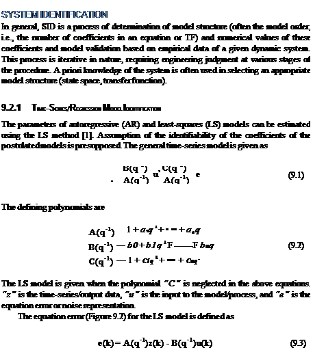
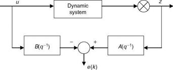
Since the data u(k) and z(k) are available from the experiments, the above equations can be put in the form

z = Hb + e (9.4)

Here, z = {z(n + 1), z(n + 2),…, z(n + N)}T with

—z(n)

—z(1)

u(n)

u(1)’

H =

—z(n + 1)

—z(2)

u(n + 1)

u(2)

(9.5)

—z(N + n — 1) ••

• – z(n)

u(N + n — 1)

.. u(N)

N is equal to the number of the data used. For example, with n = 3 and m = 1, we have

e(k) = z(k) + az(k — 1) + Я2 z(k — 2) + a3z(k — 3) — b0u(k) — bu(k — 1) (9.6)

and so on, thereby yielding, in collective form, Equation 9.4, with appropriate equivalence. Using the LS method, we get the estimates of the parameters as

b = {fib…, fin. fib…, bm} = (HTH)—1 HTz (9.7)

The coefficients of time-series models can be estimated using the SID toolbox of MATLAB. An example of human operator modeling using the time-series approach is given in Chapter 10. The covariance matrix of parameter-estimation error is given as

cov(b — b) « s2(HTH)—1 (9.8)

Here, sr2 is the estimation-residual variance.

In aircraft parameter estimation, a general form of the model to be identified occurs as

y(t) = bo + btxt(f) H———— E bn—1xn—1(t) + e(t) (9.9)

dynamic system; in fact, some intermediate steps might be required to compute y from x. This is true for aircraft parameter estimation, and the intermediate compu­tations will involve all the known constants and variables like xt and y. It is necessary to determine the parameters that should be retained in the model and estimated. This problem is handled using model order determination criteria and the LS method for parameter estimation. In aircraft parameter estimation, often y(t) represents the aerodynamic coefficients (Chapter 4) and b the aerodynamic derivatives.

Non-Model-Based Approach

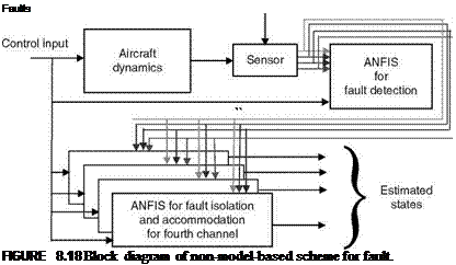
A non-model-based approach for sensor fault detection, isolation, and accommoda­tion is shown in Figure 8.12. The scheme uses the ANFIS system. The MATLAB – based functions ‘‘GENFIS’’ and ‘‘ANFIS’’ (adaptive neurofuzzy inference system) can be used to build the state observers to estimate the state pertaining to the longitudinal motion of aircraft considered. The first part consists of the state observer for each measurement channel for fault detection and isolation [12]. Each observer is trained using (uc) as the control input and measurement (e. g., pitch rate) and the corresponding true state as the output. For the purpose of detection, thresholds are computed using Monte Carlo simulation of random noises (one can use 1000 runs). The second part is for fault reconfiguration, and one can use four observers with each one trained using (uc) as the control input, the measurements from three channels (excluding a channel for which the state is estimated), and the estimated state corresponding to the measurement of the excluded channel as the output. For example, for faulty pitch rate (q) accommodation, inputs to observer are uc, w, u, and U.

image168,image169,image170

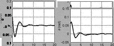
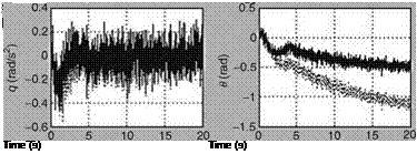
FIGURE 8.17 Comparison of states of unimpaired, impaired, and reconfigured states of an aircraft.

Example 8.7

Подпись: Faults FIGURE 8.18 Block diagram of non-model-based scheme for fault.

Realize the non-model-based sensor fault detection scheme of Figure 8.18 in MATLAB based on the foregoing theory. Use the same state-space models used in Examples 8.5 and 8.6.

image172

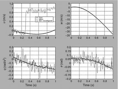
FIGURE 8.19 Comparison of true, measured, estimated state (reconfigured).

Solution

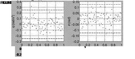
The simulation is carried out as per Example 8.5 (ExampleSolSW/Example8.7ANFIS). The minimum and maximum values of the noises were computed for each run and then the averaged value of all the runs was considered as the threshold for the purpose of detection. The sensor fault is introduced only to forward velocity u at the 31st data point by adding a constant bias of 4 m/s. The fault was detected around the 32nd data point and most of the time the fault was in the first channel. In between it went to other values but only for a single time-point and the reason for this could be a false alarm. Figure 8.19 illustrates reconfigured estimated states compared with measured (including faulty u), true, and reconfigured estimate states. In the case of faulty measurement, it is observed that, overall, the estimated value closely matches with true except at some points where the scheme is affected, perhaps due to a false alarm. Figure 8.20 shows the residuals compared with the threshold used in fault detection and isolation for each channel.

It is observed for faulty channel (i. e., u) that after reconfiguration the error lies within the threshold.

EPILOGUE

In this chapter and Appendix C, we have introduced some fundamental aspects that are important for design and analysis of flight control and reconfiguration control systems. The subject of design of flight control laws is highly specialized; hence it is not treated here. It would need a separate volume in its own right. Robustness issues, feedback properties, and classical and modern synthesis for multivariable feedback control design are surveyed in Refs. [13-15]. Evaluation of flight-control systems

image173
using the stability margins and low-order equivalent systems is discussed in Ref. [16]. Applications of ANNs and artificial intelligence to sensor fault management, restructurable control systems, and decision and control are dealt with in Refs. [17-19]. In Ref. [20], the authors develop physical insights into the relation between the singular values and the aircraft and controller dynamics by using the literal approximate factors and provide a procedure for the determination of the most important parameter uncertainties for aircraft and controllers. The idea is to obtain approximate relations for transfer function poles and zeros literally in terms of the stability and control derivatives of the atmospheric vehicle. In Ref. [21] the authors deal with the application of online parameter estimation for a restructurable control system. In Ref. [22], the authors discuss the issues and applications of evolutionary algorithms and hybrid neural and fuzzy control schemes.

Reconfiguration Concept

The technique used is known as pseudo-inverse or control mixer. The dynamics of an unimpaired closed loop system is given by

x = Ax + Buc = Ax + B(—Kx) = (A — BK)x (8.33)

Here, K is the gain matrix and is designed in such a way that eigenvalues of (A — BK) are in the left half of s-plane. The gain K can be computed using MATLAB function ‘‘LQR ()’’ and tuning its parameters by trial-and-error method until it gets the desired response from the system. In the case of the impaired system, the reconfigured closed loop dynamics is given by

x = Ax + Buc = Ax + B(—Kx) = (A — B Ki)x (8.34)

In order to achieve a nearly similar response from the reconfigured impaired system, the RHS of Equation 8.34 should be made equal to RHS of Equation 8.33, i. e.,

Подпись: (8.35)A — BK = A — BKi
BK = BKi

The gain matrix for the impaired system can be computed from Equation 8.35

Ki = (B)#BK (8.36)

Here, # is the pseudo-inverse of control vector parameters of B estimated using augmented EKF.

Example 8.6

Подпись: (8.37)

Realize the actuator fault detection scheme of Figure 8.11 in MATLAB based on the foregoing theory.

image163

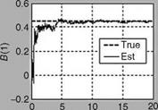
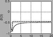
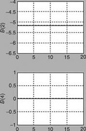
The rest of the equations used in augmented EKF are the same as those used in the scheme of Example 8.5 (ExampleSolSW/Example8.6AFDIA). The estimated value of the control vector is subsequently used for reconfiguration of impaired aircraft. For evaluation of this scheme, the fault in the actuator is introduced at the 100th iteration by changing the third element of control input vector B from its actual value of —0.91 to —0.45, i. e., nearly 50% loss in effectiveness. Figure 8.15 shows the states correspond­ing to longitudinal motion of the aircraft for unimpaired and impaired configurations. It can be seen that the states for both the configurations are comparable up to the first 5 s and thereafter a clear difference in magnitude of state of the values can be seen. The measurements are generated using the state of impaired aircraft and subsequently used to recursively estimate the elements of input control matrix B using the scheme. For the estimation of B as an augmented state with the state pertaining to longitudinal motion, EKF is used with its initial state kept at zero and accordingly state initial error covariance is computed. The tuning parameters such as Q and R are assumed to be known precisely. Figure 8.16 illustrates the estimated values of B compared with true values. B(1) converges to the true value as the number of data increases. In the case of the faulty element B(3), initially the estimated value starts from zero and then converges to true value and when the fault occurs it slowly tries to converge to the faulty value. These estimated values are subsequently used in control reconfiguration to make the performance of the impaired aircraft close to an unimpaired one. Under the scheme, first the response of the unimpaired aircraft with state feedback and without control input (i. e., uc = 0) is realized by designing the feedback gain matrix K (Equation 8.36), using the LQR method (in MATLAB). During the analysis, it is found that with feedback gain K = [0.0886 0.0048 —0.8906 —2.1274], and closed loop or controlled response of the longitudinal state tends to zero as required. The parameters, such as feedback gain K for

Time (s) Time (s)


image165image166image167

FIGURE 8.16 Comparison of true and estimated elements of control input matrix ‘‘B’’.

unimpaired aircraft, estimated B along with true B and A, are used to reconfigure the feedback gain for impaired aircraft. Figure 8.17 compares the closed loop response of unimpaired, impaired without reconfiguration, and reconfigured impaired aircraft. It is observed from the plots that the response of the reconfigured state converges to that of the unimpaired one, thereby indicating reconfiguration of the faulty system. However, much

Sensor Fault Detection Scheme

In order to evaluate the sensor fault detection scheme, primarily only one kind of sensor fault can be considered, that is, a shift in the mean of measurement noise. For fault detection, isolation, and accommodation, extended Kalman filter (EKF) in discrete time domain is mainly used. Sensor fault detection is performed by checking the change in the mean of time series of innovation sequences computed over a window length M (usually M = 20 would suffice). The hypothesis used for fault detection is as follows:

Подпись: (8.28)Hq (no fault): b(k) < xl H (fault): b(k) > xl

Here, xl is a threshold obtained from a chi-square table for a confidence probability i = 0.95 (present case) and degree of freedom Ms = M* number of measurement channels. The statistical function b(k) is computed using the following equation:

k

b(k) = Y, nT (j)S~l(MJ) (8.29)

j=k—M+1

Once the hypothesis H1 is satisfied, the next step is to find the source of fault, i. e., the malfunctioning measurement channel. Assuming that there are total “m” channels, the algorithm to isolate the faulty channel is given by

Ho, ch (no fault in “ch” channel): bch(k) < xl, ch Hi, ch (faulty ‘‘ch’’ channel): bch(k) > xl, ch

Подпись: bch(k)
Подпись: (8.30)

Here, ‘‘ch’’ is the channel number, which varies from 1 to m and xl ch is a threshold obtained from a chi-square table for a confidence probability i = 0.95 and degree of freedom Ms ch = M — 1. The statistical function bch(k) is computed using the follow­ing equation:

Example 8.5

Realize the sensor fault detection scheme of Figure 8.10 in MATLAB based on the foregoing theory.

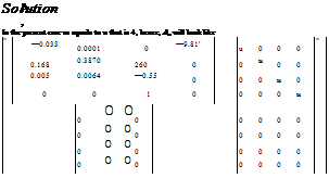
Matrices A, B, and G given here [10] can be used for generation of the data:

"—0.033

0.0001

0

—9.81

0.45

1

0

0

0

0.168

—0.3870

260

0

; в =

—5.18

; G =

0

1

0

0

0.005

—0.0064

—0.55

0

—0.91

0

0

1

0

0

0

1

0

0.00

0

0

0

1

Solution

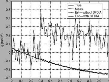
Data simulation is carried out using Equations 8.26 and 8.27 to generate the true and measured states for aircraft longitudinal motion (ExampleSolSW/Example8.5kF). Each element of “Q” is kept at 1.0e — 8, whereas, “R” under normal-sensor operation is kept at diag[0.1296 0.0009 0.0225 0.010]. In the case of SFDIA scheme, the total number of data points simulated is kept at 100 and for AFDIA 2000 data points are simulated. The control input “uc” is kept at a constant value of 8. To first evaluate SFDIA scheme, a fault is introduced in the 3rd channel (i. e., in pitch rate) measurement at the 31st second by adding a constant bias of 0.4°/s to that channel. Figure 8.12 shows the comparison of actual and faulty measurements of pitch rate for 100 data points.

image158

Time (s)

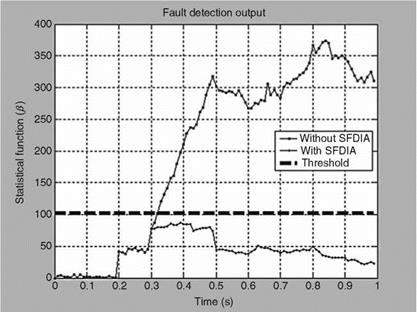
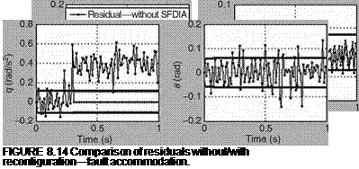
The fault detection is first carried out by comparing the statistical function b(k) with the threshold x2a selected using chi-square table. Threshold is kept at 101.88 for 20DOF and with a confidence level of 0.95. Figure 8.13 shows the comparison of b(k) with the threshold for the entire set of data points. It can be observed from the figure that fault is detected with a delay of four scans (0.04 s). The fault detection automat­ically triggers the isolation algorithm to locate the faulty channel and once the fault is located the accommodation algorithm bypasses the faulty measurements used in the state update of EKF. Figure 8.13 also compares b(k) computed for faulty and reconfigured cases. It is clear that after fault reconfiguration, b(k) never exceeds the threshold value, thereby indicating the proper handling of the faulty channel through the algorithm. The outcome of fault isolation in terms of comparison of the statistical function computed for each measurement channel with the threshold value of 31.4 for 19DOF and with a confidence level of 0.95 was that, except for the third channel, b(k) never exceeded the threshold for the remaining channels, thereby indicating the source of the fault occurrence. b(k) goes below the threshold immediately after the isolation and reconfiguration. Figure 8.14 depicts the innovation sequences along with the theoretical bounds of fSii, where S is the innovation covariance matrix and the term “i” indicates the index of diagonal elements. It can be seen from Figure 8.14 that for the faulty channel (third), the innovation sequence exceeds the bound if not reconfigured, whereas, it is forced to zero after reconfiguration. The estimated states were found to be close to the true states, thereby confirming satisfactory performance of the scheme.

image159

8.8.1 image160,image161
Actuator Fault Detection Scheme

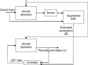
The actuator fault detection scheme is shown in Figure 8.11. The actuator fault can be modeled by multiplying the appropriate component of control vector “B” (Equa­tion 8.26) by the factor of effectiveness. The 50% loss in effectiveness means the faulty value is half of the true value. After the introduction of a fault in some of the components of control vector B, the measurements should be generated using Equations 8.26 and 8.27. The EKF filter should be reformulated as far as the plant model is concerned by augmenting the plant state with the states pertaining to components of B that have to be estimated. The reformulated plant model used in the filter is given by

~a — Aaxa (8-31)

Подпись: [A]nxn [0]mxn Подпись: [U * I]nxm [0] mxm Подпись: (8.32)

Here, the augmented state xa consists of xa — [ x B ] and the augmented matrix Aa for single control input is given by

AIRCRAFT RECONFIGURABLE/RESTRUCTURABLE CONTROL SYSTEM

A typical FTR control system would consist of actuators, sensors, computer systems, data acquisition systems, and often mechanical, hydraulic, pneumatic, electronic devices and systems [9-11]. A fault-tolerant flight-control system (FTFCS) is expected to perform the task of failure detection, identification, and accommodation of actuator and general failures. FTFCS is also useful for UAVs and MAVs. In a reconfigurable FTFCS, a full set of possible failures for different control surfaces and other probable faults is predefined. The required changes in control gains are computed offline in advance and stored in OBC for subsequent online usage. This approach requires an extensive design to consider all possible failure modes and hence a large storage space in OBC is required. In restructurable FTFCS, the required control laws are restructured online based on some identified system/fault parameters, particularly damage to a wing or control surface. ANNs and fuzzy logic find a good use for this type FTFCS. For FTFCSs, two aspects are important: (1) detection and identification of actuator fault and (2) failure accommodation. For an FBW aircraft, fault-tolerant capacity requires an increase in the number of independent control surfaces. This selection depends on: (1) control effectiveness (Cm), (2) increased aircraft complexity and cost, (3) weight constraint, (4) aerody­namic drag force, and (5) aircraft type. When any type of control surface failure occurs, the coupling between longitudinal and lateral-directional dynamics is of great concern, since this might lead to loss of stability of the vehicle. In many of these studies an accurate postfailure aerodynamic model for simulation is required. From Equation 4.6 we can guess that a damage of a control surface would cause instantaneous changes in its aerodynamic characteristics. Neglecting the effect on the axial forces, the net effect of the damage of the control surface would normally be the reduction in the relative normal force coefficient.

Sensors and actuators play a vital role in the control mechanisms of various aerospace vehicles/systems. Problems arise when a particular sensor stops working properly due to an unknown internal fault or component impairment or any cata­strophic disturbance from an external source. In that case, the whole architecture of the control system becomes hampered. There is an urgent requirement for a model that detects the failed sensor as quickly as possible and reconfigures the damaged architecture so that the controlling mechanism continues to deliver desired results without any alterations. Timely detection and adjustment of the system to cope with these uncertainties are highly desirable. This process of identification and reconfig­uration is known as sensor fault detection, isolation, and accommodation (SFDIA). The two most popular methods for SFDIA are model – and non-model-based approaches. These techniques are based on analysis of residuals between measured and predicted plant states. In the model-based technique, the algorithms commonly used are RKF (robust Kalman filter) [11], MMAE (multiple model adaptive estima­tor), and IMM (interacting multiple model). In the non-model-based approach, neural networks and fuzzy logic are used to predict the plant responses and this in conjunction with the measured states is subsequently used to detect and isolate the sensor fault. The other potential cause for hampered aircraft performance is its faulty actuator. The process of detection, isolation, and reconfiguration of actuator faults is known as AFDIA. In this case, the strategy is to pinpoint the cause of failure and then appropriately reconfigure the flight-control system such that the impaired aircraft can be made flyable.

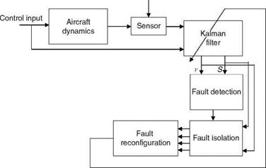
Figures 8.10 and 8.11 show the architectures used for fault detection, isolation, and reconfiguration for sensor and actuator, respectively. For data simulation, the longitudinal dynamics of aircraft control system are considered. The state-space formulation of the longitudinal motion of aircraft in continuous-time domain is as follows:

x = Ax + Buc + Gwn (8.26)

Here, x = [u, w, q, U] are the physical variables corresponding to aircraft longitudinal motion. wn is zero mean white Gaussian process noise.

Faults

image156

FIGURE 8.10 Schematic for sensor fault detection, isolation, and accomodation.

The equation used to model the sensor is given by

Zm(k) = Hx + v (8.27)

The observation matrix H is an identity matrix with the dimension 4 x 4. The measurements can be obtained with a sampling time interval T equal to 0.01 s.

Faults

image157

FIGURE 8.11 Schematic for actuator fault detection, isolation, and accomodation. (#—pseudo inverse; B—true parameters; K—feedback gain for unimpaired aircraft.)

FUZZY LOGIC CONTROL

Conventional control systems are not regarded as intelligent systems. If in conven­tional control strategy some logic is used, then it can be a start of the intelligent control system. Fuzzy logic provides this possibility. A fuzzy logic-based controller is suitable for keeping the output variables within the specified limits and also for keeping the control actuation, i. e., the control input and the related variables, within limits. In fact fuzzy logic deals with vagueness rather than uncertainty. Fuzzy logic in control would be useful if the system dynamics are slow or nonlinear, when models of the system are not available, and competent human operators are available to derive the expert rules [7]. Thus, the rule-based fuzzy system can model any continuous function or system and the quality of fuzzy approximation would depend on the quality of rules. These rules can be formed by experts and, if required, ANNs can be used to learn the rules from the empirical data. Such systems are called ANFIS (adaptive neuro-fuzzy inference system) (Chapter 9). The basic unit of the fuzzy system/approximation is the ‘‘If… Then… ’’ rule. A fuzzy variable is one whose values can be considered labels of fuzzy sets: temperature! fuzzy variable! linguistic values such as low, medium, normal, high, very high, etc. leading to membership values (on the universe of discourse, e. g., degree Celsius). The dependence of a linguistic variable on another variable can be described by means of a fuzzy conditional statement:

R: If S1 (is true), then S2 (is true) or S1 ! S2 (8.10)

image146

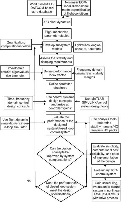
FIGURE 8.2 A typical iterative process for design of flight control.

image147

image149

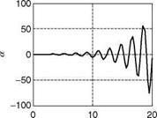
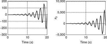
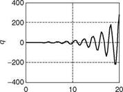
FIGURE 8.3 Time histories of aircraft with destabilized controller (Example 8.3).


image148

Подпись:R1: If S1 then (If S2 then S3) is equivalent to: R1: If S1 then R2 AND R2: If S2 then S3

The number of rules could be large (30) or for a more complex process control plant 60 to 80 rules might be required [7]. For a small task 5 to 10 rules might be sufficient like for a washing machine. Then, a fuzzy algorithm is formed by combining 2 or 3 fuzzy conditional statements: If speed error is negative large then (if change in speed error is NOT [negative large or negative medium] then change in fuel is positive large), . . . , or, . . . , or, . . . .

The knowledge necessary to control a plant is usually expressed as a set of linguistic rules of the form: If (cause) then (effect). These are the rules that new operators are trained with to control a plant, and the set of rules constitutes the knowledge base of the system. However, all the rules necessary to control a plant might not be elicited or even known. It is therefore essential to use some technique capable of inferring the control action from available rules. Forward fuzzy reasoning (Generalized Modus Ponens):

Premise 1: x is A,

Premise 2: If x is A then y is B,

Then the consequence: y is B. This is the forward data-driven inference, used in all fuzzy controllers, i. e., given the cause infer the effect. The directly related to backward goal-driven inference mechanism, i. e., infer the cause that leads to a particular effect, is as follows:

Generalized Modus Tollens:

Premise 1: y is B,

Premise 2: If x is A then y is B,

Then the consequence: x is A. Reasons for use of fuzzy control are (1) for a complex system! the math model is hard to obtain, (2) it is a model-free approach, (3) human experts can provide linguistic descriptions about the system and control instructions, (4) fuzzy controllers provide a systematic method to incorporate the knowledge of human experts, and (5) it reduces the design iterations and simplifies the design complexity. It can reduce the hardware cost and improve the control performance, especially for the nonlinear control systems. The assumptions involved in a fuzzy logic control system are [7] (1) the plant is observable and controllable, (2) expert linguistic rules are available or formulated using engineering common sense, intuition, or an analytical model, (3) a solution exists, (4) it is sufficient to look for a good enough (approximate reasoning) solution and not necessarily the optimum one, (5) there is a desire to design a controller to the best of our knowledge and within an acceptable precision range, and (6) the problem of stability/optimality remains as an open issue. Heuristic knowledge-based control does not require deep knowledge of the controlled plant and this approach is popular in the industry and manufacturing environment where such knowledge is lacking. It is case dependent and does not resolve the issue of overall system’s stability and performance. Model-based fuzzy control (MBFC) combines the fuzzy logic and theory of modern control; especially the known model of the plant can be used. This approach is useful in the control of high-speed trains, in robotics, helicopters, and flight control. In the classical gain scheduling control, the control gains are computed as a function of some variable, e. g., the dynamic pressure at flight conditions. Fuzzy gain scheduling (FGS) is a special case of MBFC and uses linguistic rules and fuzzy reasoning to determine the control laws at various flight conditions. The issues of stability, pole placement, and closed loop dynamic behavior are resolved using the conventional and modern control approaches.

Tagaki and Sugeno (TS) [7] controller is defined by a set of fuzzy rules. These rules specify a relation between the present state of the dynamic system and its model and the corresponding control law with a general rule! R: If (state) Then (fuzzy plant/process model) AND (fuzzy control law).

Let the dynamic system be given as

X(t) = f (x, u); x(0) = X0 (8.12)

Define the fuzzy state variables for the discrete case as

fXj = Y^ mfXij(x)/x (8.13)

Each element of the crisp state variable is fuzzified and in each fuzzy region of fuzzy state-space the local process model is defined:

One example of fuzzy process rules is given in Example 8.4. The process rules can be given in terms of the elements of the crisp process state. The process is specified by the state space with the degrees of fulfillment of the local models of the process employing Mamdani rule.

Подпись:x1 = mS (x)fi(x, u)

= min(mfx{ (X1),…, mfxn (Xn))fi(x, u)

The fuzzy open loop model is given as

-X = X w‘s(x)fi(x, u) (8.16)

Подпись:is the normalized degrees of fulfillment. Now the fuzzy control
Rls: if x = fxl then u = g,(x) (8.17)

In a manner similar to the development of the fuzzy open loop/process model, the control law is defined as

u = X Wc(x)gj (x) (8.18)

Here, w are the control weights. An aircraft’s dynamic characteristics would change with Mach number and altitude (or dynamic pressure). Gain scheduling is used for selecting appropriate filter (feedback controllers) characteristics (gain and time constants) so that the performance of the aircraft/control system is acceptable despite the change in its dynamics. The concept is illustrated by the following example.

Example 8.4

Use the system process rules as [7]

Подпись:R0: if xd = 0 then x = f1(x, u) = — 0.4x + 0.4u R1: if xd = 1 then x = f2( x, u) = —2.5x + 2.5u

Then

1. Obtain step responses of these two systems/process rules and compare the results.

2. Use the fuzzy gain scheduling controller concept with the following rules:

Подпись:R0: if xd = 0 then u1 = g1(x, xd) = k1(x — x^)

R1: if xd = 1 then u2 = g2(x, xd) = k2(x — xd)

Use the state feedback gains кг = 0.5 and k2 = 0.92. Then the overall fuzzy process model is given by the weighted sum:

x = wi{-0.4(x — xd) + 0.4u} + w2{—2.5(x — xd) + 2.5u} (8.21)

Design the above fuzzy gain scheduling and obtain the responses of the final system.

3. Compare the responses of the designed system with the system: x = —0.2x + 0.2u.

4. Plot all the results: step responses and Bode diagrams of the open loop and closed loop systems.

Solution

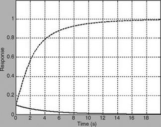
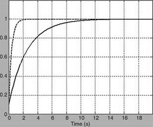
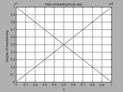
The process time constants are 2.5 and 0.4 s. The step responses of these processes are shown in Figure 8.4 (ExampleSolSW/Example8.4FuzzyControl). It is obvious from the plots that the second process rule signifies a faster process. The fading of the slow plant dynamics to the fast one is represented by the fuzzy membership functions plotted in Figure 8.5, as altitude increases. The fuzzy control law is given as

u = 0.5w1(x — xd) + 0.92w2 (x — xd) (8.22)

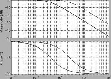
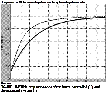
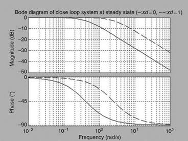
The Fuzzy controller is realized as discussed in Section 8.6, and the responses are shown in Figure 8.6. The comparison of the time responses with the invariant system is shown in Figure 8.7. The frequency responses for the open loop and closed loop systems are represented in Figures 8.8 and 8.9. The fuzzy controller meets the require­ments at both the ends as can be seen from Figure 8.7.

Response of system to unit step input (open-loop)

image150

image151

FIGURE 8.5 Gain scheduling fuzzy membership functions: Transition from slow dynamics to fast dynamics as the altitude increases.

Response of system with fuzzy feedback controller

image152

Bode diagram of open loop system (-:xd =0, —:xd = 1)

image153

Frequency (rad/s)

Подпись:

image155

FIGURE 8.9 Closed loop frequency responses of the system for two processes: At low altitude xd — 0 (- slow dynamics); at high altitude xd — 1 (— fast dynamics).

8.7 FAULT DETECTION, IDENTIFICATION, AND ISOLATION

In the present-day complex and sophisticated control systems for aerospace vehicles, the safety and reliability of the system are very important. A failure or fault could be in the hardware system or in the software. This could be due to one or more of the following: (1) design error, (2) damage, (3) deterioration, (4) EM interference, and (5) external disturbance of high magnitude. A fault could be transient, intermittent, or permanent [8]. Hence, the importance of a fault-tolerant control system in safety critical systems need not be overemphasized. The technology of fault detection, identification, and isolation in the context of a reconfigurable control system is a rapidly developing field in aerospace engineering. Due to the high demand for autonomous navigation, guidance, and control of aerospace vehicles, the subject assumes a greater significance than the basic control system. For ensuring safe flight operation of an aircraft, proper functioning of sensors, actuators, and control surfaces should be ensured. The aircraft’s flight-control systems or its subsystems should be fault tolerant to failures. Alternatively, AFCS should be adaptive and the aircraft should be able to recover from the effects of such failures. For fault detection, identification and isolation and subsequent reconfiguration, if needed, should be done in near real-time mode for it to be really effective and useful.

8.7.1 Models for Faults

behavior [9]. There are several methods and approaches based on linear and non­linear dynamic mathematical models for the analysis and design of fault-tolerant control systems (FTR). Different faults would exhibit distinct characteristics and hence naturally a multiple model approach offers a logical solution for dealing with multiple types of faults in sensors, actuators, and system dynamics. Therefore, it would be a good idea to represent each fault with a separate model, thereby enhancing the overall handling capacity of various types of faults. Based on the requirements of the system performance, multiple reference models can be defined. Once these models are defined, the fault-tolerant control system can be synthesized using the model reference approach.

Let the dynamic system be described as

X(t) = (A + Daj)x(t) + (B + Dbj)u(t) + w(t)

= Ajx(t) + Bju(t) + w(t) (8.23)

Similarly,

z(t) = Cjx(t) + v(t), j = 0, …, N —1. (8.24)

Equations 8.23 and 8.24 represent the system under normal and (N — 1) failure modes. Daj, Dbj, and Dcj define the fault-induced changes in the system dynamics, actuators, and sensors, respectively. j = 0 is a normal and nonfaulty condition. We need to specify the characteristics of the system under each fault. For this purpose, one can use the performance reduced reference model (PRRM). Let a reference model of the system under normal situation be given as

= Amxm + Bmr

(8.25)

ym стуГ v 7

When a fault occurs, the eigenvalues of PRRM would shift toward the imaginary axis, reflecting the loss of performance.

PERFORMANCE REQUIREMENTS AND CRITERIA

FBW/FCS should achieve (1) performance robustness in spite of uncertainty in plant, i. e., aircraft dynamics, and in the presence of external disturbance and (2) good command following. The FCS/control laws should also provide sufficient gain and phase margins (Appendix C) and adequate gains roll-off at high frequencies so that noise, aircraft model uncertainties, and structural modes have negligible effects on the flight/mission performance of the aircraft [5]. In most cases of design and development of a flight vehicle, especially manned aircraft, the specifications of the required handling qualities are incorporated in the design cycle. This is more so for the design of flight control laws. The time-domain and frequency-domain criteria are specified for handling qualities evaluation of the pilot-aircraft interactions (Chapter 10). At times these requirements would be conflicting in nature and some engineer­ing judgment and insights are needed to arrive at an acceptable and satisfactory design and to meet the desired goals.

8.2 PROCEDURE FOR THE DESIGN AND EVALUATION OF CONTROL LAWS

The design of flight control laws is a multidisciplinary process in which aerody­namic, structural, propulsive, and control functions are considered together. Modern flight controllers may excite structural modes of the aircraft. These modes would interact with the control-actuator dynamics. Also, because of the increasing need to integrate flight controls with engine controls, the interactions between aerodynamics, propulsive, and structural modes should be investigated and taken into account. Due to extensive use of composite (material) in the design of the airframe and control surfaces, aeroelastic coupling would also play a significant role in the design process of flight control laws.

Design and development of an FBW/FCS and autopilot presuppose a good understanding of the dynamics of the aircraft and easy availability of the mathematical models of these dynamics over the entire flight envelope (Chapters 2 through 5). Primarily, such information is available in the form of an aero database (Chapter 6),
which is usually in the form of lookup tables. These tables are constructed based on the extensive wind tunnel tests carried out on scaled (down) models of the aircraft during the design/development cycles. The database would be in terms of aerodynamic coefficients as function of several independent variables: Mach number, alpha, control surface deflection, store configurations, and any such parameter that would have major or moderate effect on these coefficients. That is, at a given flight condition (altitude, Mach number) and with the specification of other relevant parameters, one should be able to determine the values of these aerodynamic coefficients. These coefficients are used in the EOM to obtain the flight responses as discussed in Chapter 6.

A very close scrutiny of this aero database is made and the flight mechanics parameters are computed (Chapter 4) [5]. These are in terms of aerodynamic (or stability and control) derivatives and other compound derivatives; for example, the maximum roll rate is given as pmax = — 8a 2V. In a combat flight phase operation

the aircraft would have a large roll rate/However, a desired value might not be available due to limited control power and limits on the structure. In fact, dimensional linear models (Chapter 5) are obtained at several flight conditions and configurations. These models and the design specifications form a starting point for the design of control laws for the given aircraft. The design specifications could be: (1) frequency domain parameters or (2) time-domain parameters. These performance indices are collected and put in a vector form and called vector performance index, which is to be optimized. Often the structures of controller blocks (called controller transfer func­tions or filters) are specified. At times, various criteria could be of conflicting nature, and hence, some relaxation/compromise would be required in the performance of the designed system. Also, certain required constraints on the controller gains, actual control gains, and time constants (Chapter 2, Appendix C) could be specified so that these gains are not unrealizable. This process is the multi-input multi-output (MIMO) pareto-optimal or conditionally optimal control-law design procedure. In an inter­active design process, the control design engineer also simultaneously looks at the dynamic responses of the closed loop systems for checking the limits and the shape of the responses for guidance in the design process. The entire design process can be almost fully automated, thereby freeing the designer from the tedious design cycles and iterations. This is a very practical design procedure for the determination of flight control laws and can form a substantial part of the rapid prototyping formulation and computational paradigm. Hence, in general, the procedure centers around: (1) avail­ability of all the subsystem models that form the entire aircraft closed loop system, such as actuators, sensor, anti-aliasing filters, ADC/DACs, quantization errors, and computational delays (Chapter 6), (2) controller structures, and (3) closed loop system performance criteria, such as stability margins and conventional control system criteria. The computational delays can be modeled by a second-order lag TF. Often first-order TF of the form (K/(K + s)) would suffice as a model for the actuator. Controller structure could be in the form of a state space or TF. Subsystem modeling and modeling of aircraft from aero database are discussed in Chapter 6.

Subsequently, the handling qualities are evaluated and full nonlinear flight simulation (FS) is carried out. Invariably the FS is used in the flight control design cycle iterations wherein an engineer (in-the loop) would fly the simulator and perform several different types of maneuvers and failure modes and give the

assessment of the performance of the closed loop control system (aircraft and controllers). Other stages of evaluation of control laws are the following: (1) real­time simulator, (2) iron bird (and HILS-hardware in loop simulator), and (3) in-flight simulator (IFS) (Chapter 6). A comprehensive and iterative procedure [5,6] for the design of a flight-control system is depicted in Figure 8.2.

Example 8.3

The simplified block diagram of a flight-control system of a high-performance fighter aircraft is given in Figure 6.11. Use the MATLAB/SIMULINK tool to realize the interconnected blocks (Example 6.2) and vary the “destabilizing’’ gain and study the effects on the output responses.

Solution

To find the destabilizing gain, one can change each gain value individually keeping other gains invariant. From the various simulation studies (ExampleSolSW/Example8.3Control – Simu), the gain k6 is spotted as a destabilizing gain. If k6 is increased, system response becomes destabilizing, which can be seen in Figure 8.3. The simulation study is carried out with the gain k6 = 5 and all other gains are kept unaltered.