Our heavyweight helicopter equal in the world does not have
In Rostov started production of the most load-lifting rotary-wing car The Russian holding «Helicopt[...]

Everything about aircrafts and helicopters. News and events in aviation worldwide. Civil, transportation, military helicopters and airplanes.

Everything about aircrafts and helicopters. News and events in aviation worldwide. Civil, transportation, military helicopters and airplanes.

Everything about aircrafts and helicopters. News and events in aviation worldwide. Civil, transportation, military helicopters and airplanes.

Everything about aircrafts and helicopters. News and events in aviation worldwide. Civil, transportation, military helicopters and airplanes.


Recurrent neural networks (RNNs) are NWs with feedback of output to the internal states [19]. RNNs are more suitable for the problem of parameter estimation of linear dynamic systems, than FFNNs. RNNs are dynamic NWs that are amenable to explicit parameter estimation in state-space models [4]. Basically RNNs are a type of Hopfield NWs (HNN) [19]. One type of RNN is shown in Figure 2.18, the dynamics of which are given by [20]
xi(t) = —Xi(t)R 1 + ^2 wybj(t) + Ьг; j = 1,…, n j=i
|
FIGURE 2.18 A block schematic of RNN dynamics. |
b = f(x), (6) R is the neuron impedance, and (7) n is the dimension of neuron state. FFNNs and RNNs can be used for parameter estimation [4]. RNNs can be used for parameter estimation of linear dynamic systems [4] (Chapter 9) as well as nonlinear time-varying systems [21]. They can also be used for trajectory prediction/matching [22]. Many variants of RNNs and their interrelationships have been reported [20]. In addition, the trajectory matching algorithms for these variants are given in Ref. [22]; these algorithms can be used for training RNNs for nonlinear model fitting and related applications (as done using FFNNs).
The back propagation algorithm is a learning rule for multilayered NWs [17], credited to Rumelhart and McClelland. The algorithm provides a prescription for adjusting the initially randomized set of synaptic weights (existing between all pairs of neurons in each successive layer of the network) to minimize the difference between the network’s output of each input fact and the output with which the given input is known (or desired) to be associated. The back propagation rule takes its name from the way in which the calculated error at the output layer is propagated
backwards from the output layer to the nth hidden layer, then to the njth hidden layer, and so on. Because this learning process requires us to ‘‘know’’ the correct pairing of input-output facts beforehand, this type of weight adjustment is called supervised learning. The FFNN training algorithm is described using the matrix/ vector notation for easy implementation in PC MATLAB. Alternatively, the NN tool box of MATLAB can be used.
The FFNW has the following variables:
1. u0 as input to (input layer of) the network
2. щ as the number of input neurons (of the input layer) equal to the number of inputs u0
3. nh as the number of neurons of the hidden layer
4. n0 as the number of output neurons (of the output layer) equal to the number of outputs z, v), W1 = nh x n; as the weight matrix between input and hidden layers
5. W10 = nh x 1 as the bias weight vector
6. W2 = n0 x nh as the weight matrix between hidden and output layers
7. W20 = n0 x 1 as the bias weight vector
8. m as the learning rate or step size
The algorithm is based on the steepest descent optimization method [4]. Signal computation is done using the following equations, since u0 and initial guesstimates of the weights are known.
![]()
![]() У1 = W1u0 + W10
У1 = W1u0 + W10
U1 = f( У1)
Here, У1 and u1 are the vector of intermediate values and the input to the hidden layer, respectively. The f(y1) is a sigmoid activation function given by
Here, l is a scaling factor to be defined by the user.
The signal between the hidden and output layers is computed as
У2 = W2U1 + W20 (2.26)
U2 = f( У2) (2.27)
A quadratic function is defined as E = 1 (z — u2)(z — u2)T, which signifies the square of the errors between the NW output and desired output. u2 is the signal at the output layer and z is the desired output. The following result from the optimization theory is used to derive a training algorithm:
The expression for the gradient is based on Equations 2.26 and 2.27:
@E T
=-Ay2)(z – U2)uT (2.29)
Here, uj is the gradient of y2 with respect to W2. The derivative f of the node activation function is given from Equation 2.25 as
The modified error of the output layer is expressed as
![]() Є2Ь = f ( y2)(z – U2)
Є2Ь = f ( y2)(z – U2)
Finally, the recursive weight update rule for the output layer is given as
W2(i + 1) = W2(i) + me2buT + V[W2(i) – W2(i – 1)] (2.32)
V is the momentum factor used for smoothing out the (large) weight changes and to accelerate the convergence of the algorithm. The back propagation of the error and the update rule for W1 are given as
еіь = f (yi)WTe2b (2.33)
Wi(i + 1) = Wi(i) + теїьиТ + V[Wi(i) – Wi(i – 1)] (2.34)
The data are presented to the network in a sequential manner repeatedly but with initial weights as the outputs from the previous cycle until convergence is reached. The entire process is recursive-iterative.
The Feed Forward Neural Network (FFNN) is an ANN with noncyclic type NW and layered topology and no feedback. FFNN is an information-processing system consisting of a large number of simple processing elements. FFNN can be considered as a nonlinear black box (because of its model structure but not in the conventional sense of polynomial or TF model), the parameters (weights) of which can be estimated by conventional optimization methods. A typical FFNN topology is shown in Figure 2.17. FFNNs are suitable for system identification, time-series modeling, parameter estimation, sensor failure detection, and related applications
[4,15] . The chosen FFNN is first trained using the training set data and then used for prediction using another input set that belongs to the same class of data. This is the validation set [4]. The process is similar to the one used as cross-validation in system identification literature.
Computationally neural nets are a radically new approach to problem solving. The methodology can be contrasted with the traditional approach to artificial intelligence (AI). Although the origins of AI lay in applying conventional serial-processing techniques to high-level cognitive processing like concept formation, semantics, symbolic processing, etc. (in a top-down approach), the neural nets are designed to take the opposite: the bottom-up approach. The idea is to have a human-like reasoning emerge on the macroscale. The approach itself is inspired by such basic skills of the human brain as its ability to continue functioning with noisy and/or incomplete information, its robustness or fault tolerance, its adaptability to changing environments by learning, etc. Neural nets attempt to mimic and exploit the parallel processing capability of the human brain in order to deal with precisely the kinds of problems that the human brain is well adapted for [16].
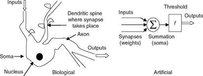
ANNs are new paradigms for computations and modeling of dynamic systems. They are modeled based on the massively parallel (neuro-) biological structures found in brains [16]. ANN simulates a highly interconnected parallel computational structure with relatively simple individual processing elements called neurons. The human brain has 10-500 billion neurons and about 1,000 main modules with 500 NWs and each such NW has 100,000 neurons [16]. The axon of each neuron connects to several hundred or thousand other neurons. The neuron is a basic building block of a nervous system. Comparison of a biological neuron and an ANN is shown in Table 2.3 and Figure 2.13.
The equivalence of the neuron process to an electronic circuit is discussed here. The voltage amplifier simulates a cell body; the wires represent the input (dendrites) and output (axon) structures. The variable resistors model the synaptic weights and the sigmoid function is the saturation characteristic of the amplifier. It is apparent from the foregoing that, for ANN, a part of the behavior of real neurons is used and ANN can be regarded as multi-input nonlinear device with weighted connections. The cell body is a nonlinear limiting function, an activation step (hard) limiter (for logic circuit simulation/modeling), or an S-shaped sigmoid function for general modeling of nonlinear systems.
TABLE 2.3
Biological and Artificial Neuronal Systems
Artificial Neuronal System
• Data enter the input layer of the ANN
• One hidden layer is between input and output layers; one layer is normally sufficient
• Output layer that produces the NW’s output responses can be linear or nonlinear
• Weights are the strength of the connection between nodes
Biological Neuronal System
* Dendrites are the input branches—tree of fibers and connect to a set of other neurons—the receptive surfaces for input signals
* Soma cell body wherein all the logical functions of the neurons are performed
* Axon nerve fiber—output channel, the signals are converted into nerve pulses (spikes) to target cells
* Synapses are the specialized contacts on a neuron, and interface some axons to the spines of the input dendrites; can enhance/dampen the neuron excitation
ANNs have found successful applications in image processing, pattern recognition, nonlinear curve fitting/mapping, flight data analysis, adaptive control, system identification, and parameter estimation. In many such cases ANNs are used for prediction of the phenomena that they have learnt earlier by way of training from the known samples of data. They have good ability to learn adaptively from the data. The specialized features that motivate the strong interest in ANNs are as follows:
1. NW expansion is a basis (recall Fourier expansion/orthogonal functions as basis for expression of time-series data/periodic signals).
2. NW structure extrapolates in adaptively chosen directions.
3. NW structure uses adaptive bases functions—the shape and location of these functions are adjusted by the observed data.
 |
neuron neuronal model
4. NW’s approximation capability is good.
5. NW structure is repetitive in nature and has advantage in HW/SW implementations.
6. This repetitive structure provides resilience to failures. The regularization feature is a useful tool to effectively include only those basic functions that are essential for the approximation and this is achieved implicitly by stopping rules and explicitly by imposing penalty for parameter deviation.
Conventional computers based on Von Neumann’s architecture cannot match the human brain’s capacity for several tasks like: (1) speech processing, (2) image processing, (3) pattern recognition, (4) heuristic reasoning, and (5) universal problem solving. The main reason for this capability of the brain is that each biological neuron is connected to about 10,000 other neurons and this in turn gives it a massively parallel computing capability. The brain effectively solves certain problems that have two main characteristics: (1) these problems are generally ill-defined and (2) they usually require a large amount of processing. The primary similarity between the biological nervous system and ANN is that each system typically consists of a large number of simple elements that learn and are collectively able to solve complicated and ambiguous problems. It seems that a ‘‘huge’’ amount of ‘‘simplicity’’ rules the roost.
Computations based on ANNs can be regarded as ‘‘sixth-generation computing’’ or as a kind of extension of massively parallel processing (MPP) of ‘‘fifth-generation computing’’ [17]. MPP super computers give higher throughput per money value than conventional computers for the algorithms within the domain of programming constraints of such computers. ANNs can be considered as any general-purpose algorithm within the constraints of such sixth-generation hardware. The human brain lives within essentially the same sort of constraints. ANN applications for large and more complex problems become more interesting. One can develop new generations of ANN design providing new learning-based capabilities in control and system identification. These new designs could be characterized as extensions or as an aid to existing control theory and new general control designs compatible with ANN implementation. One can exploit the power of new ANN chips or optical HW, which extend the ideas of MPP, and reduced instruction sets down to a deeper level permitting orders of magnitudes more throughput per money value.
There are mainly two types of neurons used in NWs: sigmoid and binary. In sigmoid neurons the output is a real number. The sigmoid function (see Figure 2.14) often used is
|
|
|
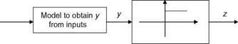
FIGURE 2.15 Binary neuron model. |
z = 1/(1 + exp(-y)) = (1 + tan h(y/2))/2
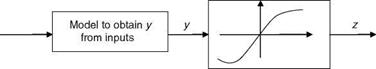
y could be a simple linear combination of the input components or it could be the result of some more complicated operations: y = summation of (weights * x) – bias! y = weighted linear sum of the components of the input vector and the threshold. In a binary neuron the nonlinear function (see Figure 2.15) is
z = saturation(y) = {1 if y >= 0} and {0 if y < 0}.
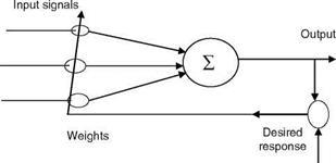
Here also, y could be a simple linear combination of the input components or it could be the result of more complicated operations. The binary neuron has saturation/hard nonlinear function. This type of binary neuron is called a peceptron. One can have a higher-order perceptron where the input y is a second-order polynomial (as a function of input data). A basic building block of most ANNs and adaptive circuits is the adaptive linear combiner (ALC) shown in Figure 2.16. The inputs are weighted by a set of coefficients and the ALC outputs a linear combination of inputs. For training, the measured input patterns/signals and desired responses are presented to the ALC. The weight adaptation is done using the LMS algorithm (Widrow-Hoff delta rule), which minimizes the sum of squares of the linear errors over the training set [18]. More useful ANNs have MLPNs with an input layer, one or at most two hidden layers and an output layer with sigmoid (nonbinary) neuron in each layer. In this NW, the input/output are real-valued signals/data. The output of MLPN is a differential function of the NW parameters. This NW is capable of approximating arbitrary nonlinear mapping using a given set of examples. For a fully connected
|
|
Inputs
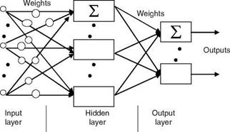 FIGURE 2.17 FFNN topology.
MLPN, 2-3 layers are generally sufficient. The number of hidden layer nodes should be much less than the number of training samples. An important property of the NW is the generalization property, which is a measure of how well the NW performs on actual problems once training is completed. Generalization is influenced by the number of data samples, the complexity of the underlying problem, and the NW size.
The usual assumption is that noise is a white and Gaussian process. White noise has theoretically infinite bandwidth and it is an unpredictable process and hence has no model structure. It is described by a mean value and spectral density/covariance matrix. The noise affecting the system can often be considered as unknown but with bounded amplitude/uncertainty. One should search the models that are consistent with this description of the noise/error processes [13].
1.3.1 Continuous-Time/Discrete-Time White/Correlated
Noise Processes
We consider the continuous-time white noise process with the spectral density (S2) passing through a sampling process to obtain the discrete-time white noise process as shown in Figure 2.12. The output is a sequence with variance Q (a different numerical value) and is a discrete process. If the sampling time/interval is increased then, more and more of the power at more and higher frequencies of the input white process will be attenuated and the filtered process will have a finite power.
Variance — S2/sampling interval (At)
We see that as the sampling time tends to zero, the white noise sequence tends to be a continuous one and the variance tends to infinity. In reality such a process does not exist. Hence, the noise is fictitious. In practice the statistical characteristic of (continuous-time) white noise is described in terms of its spectral density, i. e., power per unit bandwidth.
If we pass uncorrelated noise signal (w) through a linear first-order feedback system, a correlated noise signal (v) is generated:
v — —fiv + w
Such correlated signal/noise process would arise in practice if the process is affected by some dynamic system, e. g., turbulence on aircraft (Appendix A) [14].

![]() White noise with
White noise with
spectral density
S-continuous process
Assume that a signal has a component that drifts slowly with a constant rate equal to b. Then the model is given as
X 1 = X2
x 2 = 0
Assume that x2 = b. The signal x1 is also called the random ramp process. In a sensor fault detection application [15], one can use the innovation sequence to detect the drift in the system/signal using this model. The point is that when a system/sensor is gradually deteriorating, in a sensor fault detection/identification/isolation scheme, and if the trend (drift) in the innovation (i. e., estimation residuals, Chapter 9) can be tracked by using the drift model, then the direction of occurrence or onset of the fault can be observed.
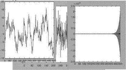 |
Generate Gaussian random noise sequence by u = randn(500,1). Then standardize the sequence by un = (u — mean(u))/std(u). The sequence u has mean = —0.0629 and std = 0.9467. The sequence un has mean = —1.8958e — 017 and std = 1. The noise sequence un is plotted in Figure 2.11a. The sequence y(k) is generated using the following steps: y(1) = 0.0 + 2* un(1); y(2) = 0.0 + un(2); for k = 3:500; y(k) = 0.9* y(k— 1) + 0.05*y(k—2) + 2* un(k); end; plot(un); plot(y) (see Figure 2.11b). The SNR = 20 log 10(var(y)/var(un)) = 31.1754. We see that the model is a stable one and hence generates a stable time series, because roots ([1 —0.9 —0.05]) are 0.9525 and —0.0525 and both are within unit circle in the z-domain/complex plane. If any one root
(b) (c)
FIGURE 2.11 (a) The noise sequence ‘‘un’’ with zero mean and std = 1.0; (b) the stable time
series y; (c) the unstable time series y.
is greater than 1, then the time series will be unstable. Generate the unstable time series by y(k) — —1.01 * y(k—1) + 0.05 * y(k—2) + 2 * un(k) (Figure 2.11c). We see that the new model is unstable and hence generates unstable time series, since roots ([1 1.01—0.05]) are —1.0573 and 0.0473 and one root is out of the unit circle in the z-complex plane.
Time series are a result of stochastic/random input to some system or some inaccessible random influence on some phenomenon, e. g., the pressure variation at some point at a certain time. A time series can be considered as a stochastic signal. Time-series models provide external description of systems and lead to a parsimonious representation of a process or phenomenon. For this class of models, accurate determination of the order of the model is a necessary step. Many statistical tests for model structure/ order are available in the literature [4]. Time-series/TF models are special cases of the general state-space models. The coefficients of time-series models are parameters that can be estimated by the methods discussed in Chapter 9. One aim of time-series modeling is its use in predicting of the future behavior of the system/phenomenon. One application is to predict rainfall runoff. The theory of discrete-time modeling is easy to appreciate. Simple models represent the discrete-time noise processes. This facilitates easy implementation of identification/estimation algorithms on a digital computer. A general linear stochastic discrete-time system/model is described here with the usual meaning for the variables in state-space form [4] as
![]() x(k F 1) = Fkx(k) + Bu(k) F w(k) y(k) = Hx(k) F Du(k) F v(k)
x(k F 1) = Fkx(k) + Bu(k) F w(k) y(k) = Hx(k) F Du(k) F v(k)
For time-series modeling, a canonical form known as Astrom’s model is given as A(q—1)y(k) = B(q—1)u(k) F C(q—1)e(k) (2.18)
Here, A, B, and C are polynomials in q—1, which is a shift operator defined as
q—ny(k) = y(k — n) (2.19)
For SISO system, we have the expanded form as
y(k) F a1y(k — 1) + ••• + any(k — n) = b0u(k) F b1u(k — 1) + ••• + bmu(k — m)
+ e(k) + C1 e(k — 1) + ••• + Cpe(k — p)
(2.20)
Here, y is the discrete-time measurement sequence, u is the input sequence, and e is the random noise/error sequence. We have the following equivalence:
A(q—1) = 1 + aq—i H—– F anq—n
B(q—1) = b0 F b1q—1 F ••• F bnq~m (2.21)
C(q *) = 1 F cq 1 F ••• F Cnq p
that first – and second-order statistics are not dependant on time “t” explicitly. These models are called time-series models because the observation process is considered as a time-series of data that has some dynamic characteristics, affected usually by unknown random processes. The input should be able to excite the modes of the system. The input, deterministic or random, should contain sufficient frequencies to excite the dynamic system to ensure that the output has sufficient effects of the mode characteristics. This will ensure the possibility of good identification. Such an input is called persistently exciting. It means that the input signal should contain sufficient power at the frequency of the mode to be excited. The bandwidth of the input signal should be greater (broader) than that of the system.
The TF form is given by
This model can be used to fit time-series data that arise out of some system/ phenomenon with a controlled input U and a random excitation. Many special forms of Equation 2.22 are possible [4,9].
Example 2.11
Expand the TF of Example 2.4 into a time-series model. Also, obtain the poles and zeros of the TF.
![]() 3z2 + 4z
3z2 + 4z
z3 – 1.2z2 + 0.45z – 0.05
Solution
We use the complex variable z for denoting the Z-transform (in discrete domain). It must be noted here that q and z are interchangeably used in the literature. Interestingly enough the variable z is, in fact, a complex variable and can represent a complex frequency parameter in z-domain. Use the forward shift operator zny(k) — y(k + n) to obtain
y(k + 3) – 1.2y(k + 2) + 0.45y(k + 1) – 0.05y(k) — 3u(k + 2) + 4u(k + 1) y(k + 3) — 1.2y(k + 2) – 0.45y(k + 1) + 0.05y(k) + 3u(k + 2) + 4u(k + 1)
Use roots ([3 4 0]) to get zeros as 0, -1.333 and roots ([1 -1.2 0.45 -0.05]) to obtain the poles as 0.20, 0.50 ± 0.0i. We see that the poles lie within a circle of radius z — 1 indicating that the model is a stable system (Appendix C).
Example 2.12
Generate a time series y using the equation y(k – 2) — 0.9y(k – 1) + 0.05y(k) + 2u(k). Let u(k) be a random Gaussian (noise) sequence with zero mean and unit standard deviation. Compute SNR as 20 log 10(var(y)/var(u)) (in MATLAB).
The following type of the state-space model can, in general, describe a continuoustime nonlinear dynamic system:
![]() X — f(x, t, b) + u + w z — h(x, b, K) + v
X — f(x, t, b) + u + w z — h(x, b, K) + v
Here, x is the (nx 1) state vector, u is the (px 1) control input vector, z is the (тех 1) measurement vector, w is a process noise with zero mean and spectral density (matrix), Q, and v is the measurement noise with zero mean and covariance matrix R. The unknown parameters are represented by vectors b and K; x0 is a vector of initial conditions x(t0) at t0. This model is highly suitable for representing many real – life systems, since they are nonlinear. The nonlinear functions f and h are vectorvalued relationships and assumed known for the analysis. Several real-life examples of this form will be seen in Chapters 3 and 9.
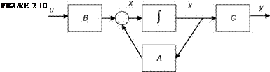
As we said earlier the state-space representation is not unique; we consider four major representations here [2]. These representations would be useful in certain optimization, control design, and parameter-estimation methods.
2.2.2.1.1 Physical Representation
A state-space model of an aircraft has the states as actual response variables like position, velocity, accelerations, Euler angles, flow angles, and so on (Chapter 3, see Appendix A). In such a model the states have physical meaning and they are measurable (or computable from measurable) quantities. State equations result from physical laws governing the process, e. g., aircraft EOM based on Newtonian mechanics, and satellite trajectory dynamics based on Kepler’s laws. These variables are desirable for applications in which feedback is needed, since they are directly measurable; however, the use of actual variables depends on a specific system.
Example 2.7
Let the state-space model of a system be given as
|
‘ — 1.43 |
(40 — 1.48)’ |
x + |
—6.3 |
|
0.216 |
—3.7 |
—12.8 |
Let C = an identity matrix with a dimension of 2 and D = a null matrix. Study the characteristics of this system by evaluating the eigenvalues.
Solution
The eigenvalues are eig(A) = 2.725, —4.995. This means that one pole of the system is on the right half of the complex s plane, thereby indicating that the system is unstable (Appendix C). If we change the sign of the term (2,1) of the A matrix (i. e., use —0.216) and obtain the eigenvalues, we get eig(A) = —1.135 ± 1.319. Now the system has become stable, because the real part of the complex roots is negative. The system has damped oscillations, because the damping ratio is 0.652 (obtained by using damp(A), and the natural frequency of the dynamic system is 1.74 rad/s). In fact this system describes the short period motion of a light transport aircraft. The elements of matrix A are directly related to the dimensional aerodynamic derivatives (Chapter 4). In fact the term (2,1) is the change in the pitching moment due to a small change in the vertical speed of the aircraft (Chapter 4). For the static stability of the aircraft, this term should be negative. The states are vertical speed (w m/s) and the pitch rate (q rad/s)
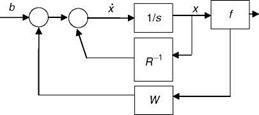
and have obvious physical meaning. In addition, the elements of matrices A and B have physical meaning, as shown in Chapter 5. A block diagram of this state-space representation is given in Figure 2.10.
Writing the detailed equations for this example we obtain
![]() w — — 1.43w + 38.52q — 6.3Se q — Q.216w — 3.7q — 12.8de
w — — 1.43w + 38.52q — 6.3Se q — Q.216w — 3.7q — 12.8de
We observe from the above equations and Figure 2.10 that the variables w and q inherently provide some feedback to state variables (w, q) and hence signify internally connected control system characteristics of dynamic systems.
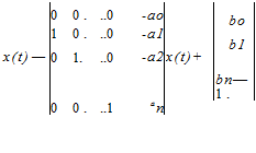
2.2.2.1.2 Controllable Canonical Form
In this form, the state variables are the outputs of the integrators (in the classical sense of analog computers, which are now almost obsolete). The inputs to these integrators are differential states (x, etc.). They can be easily obtained from a given TF of the system by inspection:
(2.12)
The corresponding TF is
![]()
 |
CmSm + Cm—1Sm 1 + • •• + C1S + CQ
sn + an— 1sn 1 ^•••^ a1s ^ aQ
One can see that the last row of matrix A of Equation 2.1 is the denominator coefficients in the reverse order. This form is so called since this system (model) is controllable, as can be seen from Example 2.8.
Example 2.8
Let the TF of a system be given as
2s2 + 4 s + 7
s3 + 4s2 + 6s + 4
Obtain the controllable canonical state-space form from this TF. Solution
Let y(s)/u(s) = (2s2 + 4s + 7) -3——– 2 ————
‘ s3 + 4s2 + 6s + 4
y(s)/u(s) — (2s2 + 4s + 7)v(s)/u(s) Hence, y(s) — (2s2 + 4s + 7)v(s) and equivalently we have
y(t) — 2€ + 4V + 7v
We define: v — x1, V — x2, and V — x3 and we get
y(t) — 2×3 + 4×2 + 7×1
![]() and x 1 — x2 and x2 — x3. Also, we have v(s) —
and x 1 — x2 and x2 — x3. Also, we have v(s) —
V — u(t) — 4V — 6V — 4v
X3 — u(t) — 4×3 — 6×2 — 4×1
Finally, in compact form we have the following state-space form:
y — [7 4 2]x
where x — [x1 x2 x3 xt].
We see that the numerator coefficients of the TF appear in the y-equation, i. e., the observation model and the denominator coefficients appear in the last row of matrix A. It must be recalled here that the denominator of the TF mainly governs the dynamics of the system whereas the numerator mainly shapes the output response. Equivalently, matrix A signifies the dynamics of the system and the vector C the output of the system. We can easily verify that eig(A) and the roots of the denominator of TF have the same numerical values. Since there is no cancellation of any pole with zero of the TF, zeros — roots ([2 4 7]).
space form as Cq — [B AB A2 B…] [2].
For the system to be controllable, the rank of the matrix Cq should be n (the dimension of the state vector), i. e., rank(CQ) — 3. Therefore, this state-space form/system is controllable, hence the name.
2.2.2.1.3 Observable Canonical Form This state-space form is given as
![]()
![]()
(2.14)
This form is so called because this system (model) is observable as can be seen from the following example:
Example 2.9
Obtain the observable canonical state-space form of the TF of Example 2.8.
Solution
We see that the TF, G(s), is given as (Exercise 2.4)
G(s) — C(sl – A)-1B
Since the TF in this case is a scalar we have [2]
G(s) — [C(sl – A)-1B}T G(s) — BT(si – AT)-1Ct G(s) — Co(sI – AT)-1Bo
Thus, if we use the A, B, C of Solution 2.8 in their ‘‘transpose’’ form we can obtain the observable canonical form:
|
0 |
0 |
-4 |
"7" |
||
|
x — |
1 |
0 |
-6 |
x + |
4 |
|
0 |
1 |
-4 |
2 |
|
u(t); y — [0 0 1]x |
The observability matrix of this system is obtained as Ob — obsv(A, C) (in MATLAB)
|
0 |
0 |
1 |
|
0 |
1 |
4 |
|
1 |
4 |
10 |
Since the rank (Ob) — 3, this state-space system is observable, and hence the name for this canonical form.
2.2.2.1.4 Diagonal Canonical Form
It provides decoupled system modes. Matrix A is a diagonal with eigenvalues of the system as the entries.
![Подпись: 11 0 0 0 ... 0- І2 ... x(t) + '1" 1 0 . . . ^n - 1 C1C2 .. cn]x(t); x(t0) — X0](/img/3131/image054.gif)
![]()
![]() (2.15)
(2.15)
If the poles are distinct then the diagonal form is possible. We see from this state – space model form that every state is independently controlled by the input and it does not depend on the other states.
Example 2.10
Obtain the canonical variable (diagonal) form of the TF
_ 3s2 + 14s + 14
y(S) — s3 + 7s2 + 14s + 8
Also, obtain the state-space form from the above TF using [A, B,C, D] — f2ss(num, den) and comment on the results.
Solution
The TF can be expanded into its partial fractions [2]:
y(s) — u(s)/(s + 1) + u(s)/(s + 2) + u(s)/(s + 4)
![]() y(t) — [1 1 1]
y(t) — [1 1 1]
 |
|
Since xi(s) — u(s)/(s + 1), we have
|
—1 |
0 |
0 |
1 |
|
|
0 |
—2 |
0 |
X + |
1 |
|
0 |
0 |
—4 |
1 |
We see from the above diagonal form/representation that each state is independently controlled by input. The eigenvalues are eig(A) as —1, —2, —4 and are the diagonal elements of matrix A. The state-space form from the given TF is directly obtained by [A, B,C, D] — f2ss([3 14 14],[1 7 14 8]) as
We see from the above results that matrix A thus obtained is not the same as the one in the diagonal form. This shows that for the same TF we get different state-space forms, indicating the nonuniqueness of the state-space representation. However, we can quickly verify that the eigenvalues of this new matrix A are identical by using eig(A) — —1,—2,—4. We can also quickly verify that the TFs obtained using the function [num, den] — ss2tf(A, B,C, D,1) for both the state-space representations are the same. The input/output representation is unique as should be the case.
In the modern control/system theory, dynamic systems are described by the state- space representation. Besides the input and output variables, the system’s model has internal states. These models are in time-domain and can be used to represent linear, nonlinear, continuous-time, and discrete time systems with almost equal ease and are applicable to SISO as well as multiple-input multiple-output (MIMO) systems. State-space models are very conveniently used in the design and analysis of control systems. They are mathematically tractable for a variety of optimization, system identification, parameter estimation, state estimation, simulation, and control analysis/design problems. TF models can be obtained easily from state-space models, and they will be unique because TF is the input/output behavior of a system. However, the state-space model from the TF model may not be unique, since the states are not necessarily unique. This means that internal states could be defined in several ways, but the system’s TF from those state-space models would be unique. By definition, the state of a system at any time t is a minimum set of values x1,…, xn, which along with the input to the system for all time T, T > t is sufficient to determine the behavior of the system for all (future) T > t. In order to arrive at the solution to an n-order differential equation completely, we must prescribe n initial conditions at the initial time “t0” and the forcing function for all (future times) T > t0 of interest: n quantities are required to establish the system ‘‘state’’ at t0. However, t0 can be any time of interest, so one can see that n variables are required to establish the state at any given time.
Let a second-order differential equation be given as
Let z(t) ! output
And z(t) = x1 and Z(t) = x2 be the two ‘‘states’’ of the system. Then from Equation 2.8 we have
X1 = Z (t) = x2
X2 = Z(t) = u(t) — 01×2 — «0x1 In vector/matrix form this set can be written as
In compact form we have
x = Ax + Bu; z = Cx (2.10)
with appropriate equivalence between Equations 2.9 and 2.10. The part of Equation 2.10 without the Bu term is called the homogeneous equation.
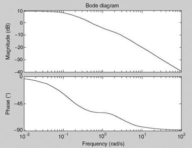
Example 2.6
Let the state-space model of a system have the following matrices [2]:
|
-2 0 1 |
1 |
|||
|
A = |
1 -2 0 |
; в = |
0 |
; C = [2 1 – 1] |
|
1 1 -1 |
1 |
Obtain the TF of this system as well as the Bode diagram.
Solution
Use the function [num, den] = ss2tf([-2 0 1; 1 -2 0; 1 1 -1], [1 0 1], [2 1 -1], [0], 1) to obtain num = [0 1.0 4.0 3.0] and den = [1.0 5.0 7.0 1.0] and hence the following TF can be easily formed:
s2 + 4 s + 3
s3 + 5s2 + 7s + 1
The Bode diagram is obtained as in Example 2.1 (see Figure 2.9). We see that the Bode diagram of this seemingly three degrees of freedom (3DOF) system looks like that of a first-order system. To understand the reason we obtain the roots of the denominator as -2.4196 + 0.6063І; -2.4196 — 0.6063І; -0.1607 and the roots of the numerator as —3.0 and -1.0. Although there is no exact cancellation of the (numerator) zero at 3.0 and the (denominator) complex pole, effectively the frequency response degenerates to that of a TF with reduced order. The eigenvalues of the system obtained by eig(A) are exactly
|
FIGURE 2.9 Bode plot of the 3DOF state-space system. |
the roots of the denominator. This example illustrates a fundamental equivalence between SISO TF and the state-space representation of a dynamic system as well as effective (though not exact) zero/pole cancellation of the TF. This example also hints at the prospect that lower-order equivalent TFs can be obtained from some higher-order TFs by some approximation methods as long as the overall frequency responses (as represented by Bode diagram) and time responses are equivalent in the range of interest.