Category FLIGHT MECHANICS MODELING and ANALYSIS

The “q’’-operator of Equation 2.4 is not like the continuous-time operator d( )/dt. If q is replaced by a “difference operator,’’ which is like a ‘‘derivative,’’ the correspondence between discrete-time and continuous-time system will definitely be better. The delta operator with t as the sampling interval is defined as [12]

8 = (2.6)

t

Table 2.1 gives equivalent TF models in various domains: d/dt = D, q or shift form, and delta form.

There is good correspondence between delta form TF (DFTF) and continuous­time system expressions (columns 1 and 3), whereas the correspondence between the continuous-time system and the shift form TF (SFTF; columns 1 and 2) is not obvious, even though these TFs are equivalent in their input/output behavior. The main point is that if we fit a DFTF to the discrete-time data, then from the DFTF we can easily discern the characteristics of the underlying continuous-time system. This cannot be done from SFTF unless it is either converted to discrete Bode diagram or time response is obtained. This is the main advantage of DFTF compared to SFTF.

Similarly DFTF can be converted to CTTF, but it will be seen that the difference between DFTF and CTTF is inherently small and the original DFTF can be inter­preted in a manner similar to CTTF, which will not be the case with SFTF in general. We emphasize here that t should be quite small.

In shift form we have

qx(k) = Fx(k) + Gu(k) y(k) = H x(k)

Then in the delta form we have

q = 1 + t5

5x = F’x + G’u (2.7)

y = H x

With

F’ = (F – I)/t; G’ = G/t; H = H

Example 2.5

Obtain the roots of the numerator (zeros) and the denominator (poles) of the model forms [12] given in Table 2.1.

Solution

The zeros and the poles are obtained by using roots ([1 1 1]), etc., as given in Table 2.2. Thus, we see a striking similarity between the poles of CTTF (rows 1, 2, 3) and DFTF (rows 7,8,9), respectively. However, the SFTFs have additionally one zero each, and there is no correspondence between poles of CTTF and SFTF. Thus, one can easily see the merits of DFTFs.

Let the system be described by the difference equation as

y(k) + a1y(k — 1) + ••• + any(k — n)

= b0u(k) + b1u(k — 1) + ••• + bmu(k — m) (2.3)

Using the time-shift operator [8], we obtain

q—1y(k) = y(k — 1)

A(q!) = 1 + aiq 1 +———– + n

B(q—1) = bo + biq~l H– h bmq~m

Thus, we have A(q—1)y(k) = B(q—1)u(k) and applying the Z-transformation we get the discrete TF (DTF/pulse TF or shift-form TF) for the discrete time-linear dynamic system:

b0 + b1Z 1 H——- H bmz m

1 + a1Z-1 +——- + a„z~"

Here, z is a complex variable, m, n (n > m) are the orders of the respective polyno­mials. The discrete Bode diagram can also be obtained. The roots of the denominator polynomial will give modes of the system in terms of frequency and damping ratio, which are important parameters to be ascertained from real flight data as first-cut results (Chapter 9). However, these are in the z domain and not in the continuous­time domain. For proper and formal interpretation, one should transform these into s-domain parameters. One major limitation of this approach is that there is no apparent correspondence between the numerical values of the coefficients of the DTF/SFTF and the corresponding CTTF of the real system. However, this corres­pondence is very closely obtained if the delta-operator form of the TF (DFTF) is employed for modeling and estimation as discussed in the sequel.

Example 2.4

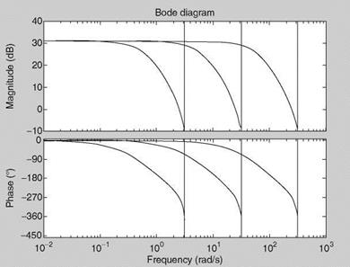
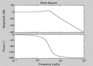
Obtain the Bode diagram for the pulse TF [2] given as

Solution

We use the function dbode([3 4 0], [1 -1.2 0.45 -0.05], 1) to obtain/plot the Bode diagram for the given discrete-time system. Here, sampling time (interval) is chosen as 1. Change the sampling time to 0.1, 0.01 and obtain the Bode diagrams (Figure 2.8).

As the sampling time reduces, the frequency range increases.

Let a system be described by a linear constant coefficient, ordinary n-order differ­ential equation:

dny(t)/dtn + я„_1 dn Vf)/df” 1 +———– h a0y(t)

= tp dpu(t)/dtp + ••• + r0u(t) (2.1)

Here, u(t) is the system input and y(t) its output. Taking the Laplace transform [2], and assuming that the initial conditions are zero, we obtain the continuous-time TF (CTTF):

y(s) = G(s) u(s)

Tpsp + tp—1 S’-1 h – h t1s + t0 (2:2)

= u(s)

sn + an-1sn 1 + ••• + a1 s + a0

Here, s is a complex (frequency) variable. This is one type of the mathematical model of a SISO system. The linear theory of analysis can be applied to this model and the system’s properties can be analytically derived from this model itself. The natural dynamic behavior of the system, in fact now of the model, can be evaluated by computing the roots of the denominator of G(s). These roots describe the various natural modes of the system, assuming that the model is nearly a good representation of the system, and dictate the amplitude and the phase of the response. If the value of n is equal to 2 then this TF is called a second-order TF and its denominator has two roots (real/complex). One can relate this to short-period modes of an aircraft wherein the short-period frequency and damping are important parameters, which are often discussed in dealing with simulation/control of aircraft (Chapter 5). These frequency and damping parameters in turn depend on certain important aerodynamic (stability and control) derivatives of the aircraft, the description of which is given in Chapter 4.

Example 2.1

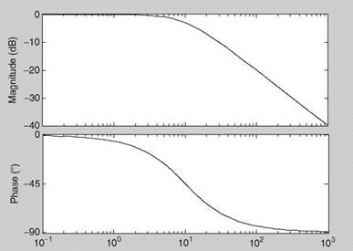
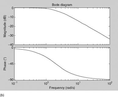
Obtain the Bode diagrams for the TF of an electrical circuit of Figure 2.3 for the time

constant of 0.1 and 0.5 s. The resistor is R Ohm and the capacitance is C microfarad.

The time constant is given as RC = t(s).

Solution

Specify numerator and denominator of the TF as num = [10], den = [1 10] (in the command window of MATLAB). Then use sys = tf(num, den) and bode(sys) to obtain/plot the Bode diagram (Figure 2.4). Repeat with 10 replaced by 2. At the cutoff

(a)

FIGURE 2.5 Mechanical spring-mass system.

frequencies (Cof, cutoff frequency = 1/time constant) the phase (lag) is —45°, the property of the first-order TF. The bandwidth (Appendix C) of the system with Cof = 10 rad/s is broader than that with Cof = 2 rad/s.

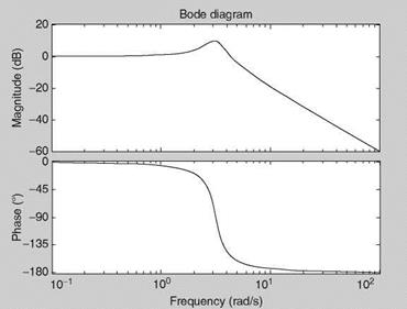
Example 2.2

The TF of a second-order mechanical system of Figure 2.5 is given as

G(s, Xs) = K/M

() f (s) s2 + (D/M)s + K/M

Here, M is the mass, D is the damping constant, and K is the spring stiffness/constant. Use suitable values for M, D, and K and obtain the Bode diagrams. Study the improvement in the damping property by increasing the value of D by a factor of 2.

Solution

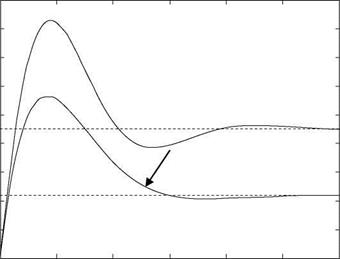
Let M = 10, D = 10, and K = 100, arbitrarily. Obtain numerator and denominator of the TF as num = [10], den = [1 10/10 100/10]. Then use sys = tf (num, den) and bode(sys) to obtain=plot the Bode diagram. We see that the natural frequency is sqrt(K/M) = 3.1623 rad/s and the damping ratio = 0.1581 (of the second-order system; Exercise 2.2), which is not the same as the damping constant. Due to low damping the magnitude of the TF has a peaking value (Figure 2.6a). Repeat the solution with D = 20 (Figure 2.6b). The increased damping constant has increased the damping ratio (the magnitude of the peak is reduced). The step responses are improved (Figure 2.6c). The step response is generated by step(sys). The first plot is held (by typing ‘‘hold’’) and then the step response with D = 20 gets automatically superimposed. We see that the time response is still not damped well. With D = 40 the response (with arrow) is very well damped and acceptable. The time constant (Appendix C) is approximately the same but the transients are suppressed when the value of D is increased. One can easily relate this TF to the short-period mode of an aircraft (Chapter 5). Thus, in the (very) approximate sense, the aircraft’s pitching motion dynamics are like a second – order spring-mass system.

Example 2.3

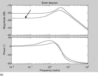
Obtain the Bode diagrams and the step responses of the following TFs [11] and comment on the results.

Solution

First, we obtain the Bode diagrams by using the steps: numl = [0.787 1.401]; deni = [1 3.785 15.49]; sysl = tf(numi, deni); bode(sysl); hold; num2 = [0.638 0.451]; den2 = [1 4.67 10.30]; sys2 = tf(num2,den2); bode(sys2) (in this sequence in the MATLAB command window). The plots are shown in Figure 2.7a. Then, we

(a)

(c)

obtain the step responses by using step(sys1); hold; step(sys2) (the plots are shown in Figure 2.7b). Next, we obtain the poles of these TFs: roots(den1) — —1.8925 ± 3.4509; roots(den2) — —2.3350 ± 2.2018. We also have the damping ratios and frequencies as

(continued)

0 0.5 1 1.5 2 2.5 3 Time (s)

(b)

FIGURE 2.7 (continued) (b) Step responses of the second-order systems (sysl; sys2 with an arrow).

damp(sys1) = 0.481, 3.94; damp(sys2) = 0.728, 3.21. We see that the second system has much better damping than the first one as is obvious from the step response of the second system (Figure 2.7b; see arrow). Actually these TFs/models are the lower-order equivalent system models (LOTF in Chapter 10) of the pitch rate to longitudinal input of F-18 HARV (high angle of attack research vehicle), identified from the measured data [11]. These LOTF models are used for evaluation and prediction of the HQs of the aircraft (Chapter 10).

Studies of electric/electronic circuits, basic linear control-systems, mechanical systems, and related analyses lend to the TF analysis [2]. For single-input single­output (SISO) linear systems, a TF is defined as the ratio of the Laplace transform of the output and that of the input. It is often important to quickly determine the frequencies and damping ratios of the dynamic systems. This is true also for aircraft modes and aircraft-control system loop TF to assess the key dynamic characteristics (the stability/gain – and phase-margins of the feedback control system; see Appendix C) for longitudinal and lateral-directional modes from small perturbation maneuvers (Chapters 5 and 9) [5]. Often this is termed as Z-transform analysis; however, we will consider it as TF analysis in which case the coefficients of numerator and denominator polynomials (in “z” or “s”—complex frequency) are estimated using a least-squares method from the real test data. This estimation can be performed to obtain either discrete time-series models (to obtain pulse TF—in z domain) or directly the continuous-time models (by using appropriate methods [10] in s domain). Additionally, one can obtain the Bode diagram, the amplitude ratio, and the phase of the TF as a function of frequency (Appendix C).

In one way, model building is closely connected to experiments and observations. This is called empirical model building. Formulation of a theory can be called ‘‘model building’’ because it gives an analytical basis to study the system. Theory is a proposed concept of the system studied, e. g., the theory of Newton’s laws of motion lends to equations of motion (EOM) of an aerospace vehicle (Chapter 3). These EOM form the basis of mathematical models of such a vehicle and are the backbone of flight control, flight simulation, parameter estimation from flight data, and handling qualities analysis (HQA). This is the process of application of basic laws of physics: force/moment balance for mechanical systems, Kirchoff’s laws/Maxwell’s electromagnetic laws for electrical/electronic systems, and energy balance for thermal and propulsion systems. Thus, model building consists of (1) selection of a mathematical structure based on knowledge of the physics of the problem, (2) fitting of parameters to the experimental data (estimation), (3) verifica – tion/testing of the model (diagnostic checks), and finally its use for a given purpose.

In most aircraft identification/estimation applications [4], the model can be represented by a set of rigid body equations in the body axis system [5]. The basic EOM, derived from Newtonian mechanics, define the aircraft characteristic motion. They are based on the fundamental assumption that the forces and moments acting on the aircraft can be synthesized. In many practical cases, the forces and moments, which include the aerodynamic, inertial, gravitational, and propulsive forces, are approximated by terms in the Taylor’s series expansion. This invariably leads to a model that is linear in parameters. Aircraft mathematical models are treated in Chapters 3 through 5. A more complete model can be justified for the correct description of aircraft dynamics. The degree of relationship between the complexity of the model and measurement information needs to be ascertained. To arrive at a complex and complete model, one would need a series of repeated experiments under various environmental conditions and a large amount of data. This will ensure the statistical consistency of the modeling results in the face of the uncertainties of measurement of noise/errors. However, how much of this additional effort/data will be useful in building the complete model will depend on the methods of reduction of the data and engineering judgment.

There are two types of models: parametric and nonparametric. In a parametric model the behavior of a system is captured by certain coefficients or parameters: state-space, time-series, and transfer-function (TF) models. The model structure is either assumed known or determined by processing the experimental data. A non­parametric model captures the behavior in terms of an impulse response or spectral density curve, and no model structure is assumed. Near equivalence is present between these two types of models, especially for linear systems (or linearized systems). Given a set of data, an approach to construct a function, y = f (x, t), is an integral part of mathematical model building. This function should be parameterized in terms of a finite number of parameters. Thus, the function ‘‘f ’’ is mapping from the set of x values to the set of y values. This parameterization could be a ‘‘tailor – made’’ [6], orthogonal function expansion, or based on artificial neural networks (ANNs) [7]. If a true system cannot be parameterized by a finite number of parameters, then one can use an expanded set of parameters as more and more data become available for analysis. This is a problem of parsimony. A set of minimum number of parameters is always preferable for good predictability by the identified model. A complex model does not necessarily mean that it is an excellent (predict­ive) model of the system. Interestingly, one can say that the exact model of a system is the system itself! The most important aspect of mathematical model building is to arrive at an adequate model that serves the purpose for which it is designed. One can look for a model that is probably approximately correct.

For tailor-made model structures, i. e., physical parameterization, it is necessary to bring physical modeling closer to system identification. This aspect is difficult to realize, since the parameters should be identifiable from the input/output data. These models are often in the form of state-space structures. These models are based on the basic principles of the system’s behavior and involve the physics of the process and are often termed as phenomenological models. The simulation of these models is complex, but they have a large validity range [6], e. g., complete simulation of the flight dynamics of an aerospace vehicle. In so-called black box models, like finite impulse response (FIR), autoregressive-exogenous (ARX) inputs, and Box-Jenkin’s models for linear systems [8], the a priori information about the system is either very little or nil. The canonical state-space models and difference equation models have parameters that have necessarily no physical meaning. These models, often called readymade models, represent the approximate observed behavior of the process. For nonlinear systems, one can use Volterra models and multilayer perceptrons (MLPNs), i. e., neural networks (NWs) [9]. Another black box nonlinear structure is formed by fuzzy models that are based on FL [7]. Since always some a priori information about a system will be available, these black box models can be considered as gray box models. Also, it is possible to preprocess the data to get some preliminary information on the statistics of the noise affecting the system, thereby leading to gray box models.

2.1 INTRODUCTION

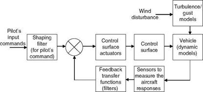
An aircraft can be considered as a dynamic system while in any type of dynamic- flight operation, since flight-related control functions to be performed are necessarily (1) the deflection of (aerodynamic) control surfaces and (2) the change in the engine thrust, which acts as input to the dynamic system, and the responses of the aircraft are the desired outputs: an equilibrium state of the aircraft’s motion, stabilized aircraft motion after a disturbance, and a change of one equilibrium state to another, if required. An aircraft is made of structures/materials, and has to have an engine for providing thrust, avionics systems, and control mechanisms; moreover, it has to ultimately fly in the air and the above-mentioned operations are called upon to be performed for any successful flight mission. Hence, the subject of flight mechanics can be and should be studied from the ‘‘control system’’ point of view. This study involves modeling and analysis of the dynamic system (in general, an atmospheric vehicle).

A study of the dynamic system can be performed via analytical or experimental means. The analytical approach yields a mathematical model based on several assumptions (because real-life dynamic systems are mostly/often nonlinear and distributed in nature) and application of the theory and concepts of modeling. In an experimental approach one has to design an appropriate experiment and generate data for analysis. This analysis is mainly carried out by using signal processing, system identification, and parameter-estimation techniques. Mathematical modeling of dynamic systems is very essential for analysis, design and simulation of control systems, and for prediction of behavior of these systems. A mathematical model characterizes the static and dynamic behavior of a system. Some practical examples are use of mathematical models in flight simulation and design of control systems for aerospace vehicles (like aircraft, rotorcraft, missile, unmanned aerial vehicles, micro­air vehicles, and spacecraft), weather forecasting, control of robotic systems, use in optimization of chemical processes in industries, and analysis of communications and biomedical signals.

A system is a set of components or functional activities that interact with each other to complete a specified task or a mission. Some examples of systems are chemical plants, robotic systems, atmospheric vehicles, computer networks, and the economy (process) of a country. Most dynamic systems are described by differential/difference equations. There is exchange or change of energy and dissi­pation in (damped) systems. A real-life dynamic system can be modeled using a mathematical model, which should be obtained, refined, and validated based on the acquired/actual data from the experiments on the system. The choice of a gross model is dictated by previous experience and the physics of the problem at hand. A fair amount of knowledge is generally accessible to the model developer/analyst. A system, in general, consists of a collection of variables needed to describe its dynamic behavior at some point in time. A system could be continuous-time or discrete-time when the state variables change either continuously or at discrete points in time (in sampled data systems), respectively. In aerospace applications, mixed – type models are used (Chapter 9). A typical atmospheric vehicle (control) system is shown in Figure 2.1. The terms system, plant, and process are used interchangeably. An aircraft can be called a system, whereas a chemical system is called a plant. This plant involves various processes for which again some mathematical models are required. A telephone/computer network can also be called a system. In many problems in science and engineering, one finds a crucial need to represent a dynamic system by its mathematical model.

This model is used for a variety of reasons: (1) to study basic dynamic charac­teristics of the system, (2) to predict future behavior of the system, e. g., weather forecasting, (3) to analyze the stability and control characteristics of the system so as to help monitor, modify, regulate, or control the behavior of the dynamic process/plant/system, e. g., chemical reactors, (4) to simulate the responses of the system for various kinds of inputs/environment, e. g., flight dynamics simulator (Chapter 6), and (5) to optimize cost and to reduce losses, e. g., dynamics of the economy of a country.

Thus, mathematical models are used in research for interpretation of acquired knowledge or measurements that provide clues for further investigations [1]; e. g., first a simplified model of the system is used and then, based on the analysis of experimental data, this model is revised. A mathematical model for the purpose of designing a new system or a controller for the same system is expressed in a manner that is compatible with the design criteria: guaranteeing the basic static/dynamic stability, overall performance, tracking error minimization, safety, and cost. For example, a time-domain model will be more suitable for use in

control-optimization methods based on time-domain methods and hence the know­ledge of components and subsystems should be in such usable forms. Finally, the control actions on a system depend on the knowledge about the system.

A mathematical model is a simplified representation of a system that helps in understanding, predicting, and possibly controlling the behavior of the system [1,2]. A model presents the knowledge about the system in a very practical form. In fact a model simulates or mimics the behavior of the system. Models could be of several types: hardware models (like the scaled model of an aircraft, a missile, or a spacecraft that is used in wind-tunnel testing), software expressions/computer algorithms, conceptual or phenomenological, physical, and symbolic models like maps, graphs, and pictures. A model represents a reality, the system, phenomenon, or process under study, with reduced complexity. Scientists and engineers all over the world make major efforts to understand the various natural phenomena as well as the properties and characteristics of man-made systems. Mathematical modeling is one of the most fascinating and intriguing fields of research. It encompasses the study of determin­istic and stochastic systems. Stochastic systems are, in general, difficult to model. Hence, a midway approach is usually preferred: deterministic systems affected by additive or multiplicative random noise.

There are three basic reasons why the usual deterministic systems/control theories do not provide a complete means of performing this analysis and design [3]:

(a) No mathematical model of a given system is perfect. Effects are modeled approximately using a mathematical model. There are many sources of uncertainty in any mathematical model of a system. Certain types of uncertainties can often be described by some random phenomena. Some uncertainties can be described by bounded but unknown disturbances that are nonrandom in nature. Between-the-events uncertainties can be axiomatically defined by probability theory, which is fundamentally based on binary or crisp logic. Within-the-events uncertainties can be modeled using the concepts of fuzzy logic (FL), which is a multivalued logic.

(b) Dynamic systems are driven not only by deterministic control inputs but also by disturbances that are neither controllable nor deterministic. Such disturbances are random and are usually modeled by the white Gaussian process. However, non-Gaussian, uniform, or other kinds of noise processes are sometimes present. Atmospheric turbulence and gust act on a flying vehicle.

(c) Measurements (sensors) do not provide perfect and complete data about a system. They introduce their own system dynamics and distortions. They are also corrupted with noise.

In the light of the above observations, the following questions become very relevant and interesting [3]: (1) What kind of models should be used to explain such uncertainties, for example, Gaussian or uniform probability distributions, or bounded disturbance models? (2) With such noisy data, how do we use the system models to optimally estimate the quantities of interest to us? System identification, state estimation, and specifically parameter estimation [4] and estimation of the spectra
of signals play an important role in analysis. (3) How do we control the system’s behavior in the face of these uncertainties, e. g., design of a suitable optimal control­ler? (4) How do we evaluate the performance of such estimators and control, for example, quality or goodness-of-fit criteria, stability (gain and phase) margins, error performance, and robustness of performance?

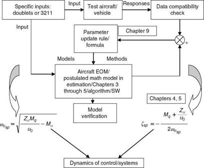
Some of the foregoing aspects are studied in the context of flight mechanics modeling and analysis in this book. A two-way approach to mathematical modeling is illustrated in Figure 2.2 [1]. The left side depicts the analytical route for model building and the right side the empirical data-based model-building route. The block diagram illustrates the comprehensive process of building a mathematical model. Most systems are nonlinear and distributed in nature: there are two independent variables—time and space. Such systems are called distributed systems and can be described by partial differential equations (PDEs). When the linearization process is accomplished, linearizing errors will occur because of approximation. If the spatial effects are lumped, then we get linear models described by ordinary differential equations (ODEs). Such systems/models are called lumped systems. At this stage we obtain a model that can be postulated for further analysis and revised based on the systematic application of the right side path. The measured data are used in system identification/parameter-estimation procedures to arrive at an adequate model struc­ture and parameters of the mathematical model [4]. This path involves measurement noise, data handling errors, quantization errors, and estimation errors.

FIGURE 2.2 A two-way approach to mathematical model building.

Chapter 2 introduces the concepts and methods of mathematical structures and model building for dynamic systems. The conventional transfer function (TF), time series, and state-space modeling aspects are treated. The delta-operator TF theory is highlighted. The new paradigms of ANNs – and FL-based modeling are also dis­cussed. Uses of many of these model types are treated in subsequent chapters appropriately.

Chapter 3 deals with the EOM of aerospace vehicles, especially for aircraft, helicopters, and missiles. The solution of these equations provides the dynamic responses of the vehicle. Aerodynamic derivatives are the kernel of the EOM. Together these models capture the dynamic behavior of the vehicle in motion. Chapter 4 discusses the fundamental concepts of aerodynamic derivatives and

▼

models. Aerodynamic derivatives as the constituents of the aerodynamic model building are explained in detail to aid in better appreciation of the material in the later chapters. Chapter 5 resorts to simplification of the EOM, since these could be complicated and nonlinear. The simplified EOMs with embedded aerody­namic derivatives provide easier and better understanding of the behavior of the vehicle. It is here that some of the concepts and methods of Chapter 2 will be useful.

Chapter 6 discusses the concepts and approach to simulation of aircraft dynam­ics. Depending on the availability of detailed models of the subsystems of aircraft, simulation could be made simpler or more sophisticated. Its use in understanding the dynamics of a flying vehicle, in validating flight-control laws, and trying out parameter-estimation exercises need not be overemphasized. Chapter 7 briefly discusses the types of input excitation signals (commands) and flight-test maneuvers, which are an integral part of the flight-test exercises of an aircraft under certifi­cation or other special test trials. It also deals with the need for flight data generation for subsequent parameter estimation in the determination of aerodynamic derivatives.

Chapter 8 deals with the principles of reconfiguration/FL control since detailed treatment of flight control deserves a separate volume. Some modeling and analysis aspects of aircraft fault detection and identification are discussed. Several important features of modeling and design processes are outlined.

Chapter 9 deals with the concepts and methods of system identification and parameter estimation as applied to flight-test data. Some important methods are discussed and results of several practical case studies are also presented. Recent aspects of analytical global modeling and neural network – and FL-based parameter – estimation approaches are treated. A quick look at the companion volume [4] (and associated MATLAB SW) would be a good idea here.

Chapter 10 deals with the concepts of HQA of aircraft and helicopters. The HQA helps in the evaluation of aircraft design (though in a limited way), its dynamic behavior, and flight-control laws at the simulation stage as well as after the flight tests. For fighter/large transport aircraft and rotorcrafts, evaluation of pilot-vehicle interactions via HQA is very important in the early vehicle development/modification programs. Aspects of HQA and pilot-induced oscillations, better known as pilot – vehicle interactions, are also discussed in this chapter.

It would be, of course, necessary to have a reasonably good background in the basics of aerodynamics, linear control systems, and linear algebra. However, several important concepts related to aerodynamics of atmospheric vehicles, statistics and probability, and systems/signal are compiled in Appendices A, B, and C to support the material of Chapters 2 through 10.

Although enough care has been taken in working out the solutions of examples/ exercises and presentation of various concepts, theories, and case study results in the book, any practical applications of these should be handled with proper care and caution. Any such endeavors would be the reader’s own responsibility. MATLAB programs developed for illustrating various concepts, via examples in the book, would be accessible to the reader.

The HQA and prediction for a fighter aircraft are important in the design and development of a flight-control system [11]. Traditionally, a pilot’s opinion ratings have been on 1- to 10-point scale, called Cooper-Harper scale. Each point gives a qualitative opinion of the pilot’s view of the aircraft’s overall behavior for a specified task/mission. This resembles multivalued description. The ratings/qualitative description is also specified in the three levels: rating 1-3.5 ! Level 1; rating 3.5-6.5 ! Level 2 and rating 6.5-10 ! Level 3. The description of the behavior of the aircraft with a pilot in the loop sounds somewhat like a rule-based logical enunciation of the pilot’s assessment of the aircraft’s performance. Levels 1-3 have a gradation more coarse than the pilot’s rating scale. To quantify this assessment, several HQ criteria have been evolved, which are largely based, in one way or the other, on the fundamental tenets/concepts of the (conventional) control theory, e. g., bandwidth, rise time, settling time, gain and phase margins (GPMs), etc. [12]. It might perhaps be feasible to establish some connectivity between multivalued FL/S, H-infinity concept, and HQ criteria. FL/Ss are useful in representing, in some concrete form, the uncertainty in a system’s model—this uncertainty plays an important role in evaluating the robustness of a flight-control system—the stability and related aspects of which are evaluated using the HQ criteria. A possible systems-oriented synergy of many such aspects presented in this book is highlighted in Figure 1.3 [13]. Further systems-oriented synergy is depicted in Figure 1.4.

Thus, the important features of flight mechanics/dynamics are prediction, mea­surements, and representation, i. e., modeling and analysis of aerodynamic forces, and evaluation of HQ. Related main problems in engineering are [2,6,14,15,17] (1) stability in motion, (2) responses of the vehicle to propulsive and control input changes, (3) responses to atmospheric turbulence and gust, (4) aeroelastic oscilla­tions like flutter, and (5) performance in terms of speed, altitude, range, and fuel assessed from flight maneuvers and testing. Reference [15] is a recent volumetric treatise on flight dynamics. Also, the field of ‘‘soft’’ computing [16] is gaining importance in the aerospace field and hence some aspects are dealt with in this volume (Chapters 2, 8, and 9). There is an immense scope of extending soft computing to flight simulation (ANN—polynomial models for aero data base repre­sentation), human operator modeling, etc.

FIGURE 1.3 System synergy of aircraft control system aided by ANNs, fuzzy system (FS), system identification (SID) and restructuring schemes (AGS: adaptive gain scheduling). (From Raol, J. R., ARA Journal, 2001, 25, 2002. With permission.)

FL is also emerging as a new paradigm for nonlinear modeling, especially to represent certain kinds of uncertainty with more rigor [9,10]. FL-based systems have the following features: (1) they are based on multivalued logic as against bivalued (crisp) logic, (2) they do not have any specific architecture like neural networks, (3) they are based on certain rules that need to be a priori specified, (4) FL is a machine-intelligent approach in which desired behavior can be specified by the rules through which an expert’s (design engineer’s) experience can be captured, (5) FL/S deals with approximate reasoning in uncertain situations where truth is a matter of degree, and (6) a fuzzy system is based on the computational mechanism (algorithm) with which decisions can be inferred in spite of incomplete knowledge. This is the process of the inference engine. FL-based control is suitable for multi­variable and nonlinear processes. The measured plant variables are first fuzzified. Then the inference engine is invoked. Finally, the results are defuzzified to convert the composite membership function of the output into a single crisp value. This specifies the desired control action. Heuristic fuzzy control does not require deep knowledge of the controlled process. Heuristic knowledge of the control policy should be known a priori.

There are several ways in which FL can be used to augment the flight-control system: (1) simulating pilot response to an aircraft that is not behaving as expected due to damage or failure, (2) incorporating complex nonlinear strategies based on the pilot’s or system design engineer’s inputs within the control law, (3) performing adaptive fuzzy gain scheduling (AGS) using the fuzzy relationships between the scheduling variables and controller parameters, and (4) in FL-based adaptive tuning of the Kalman filter for adaptive estimation/control.

ANNs are emerging paradigms for solving complex problems in science and engin­eering [7-10]. ANNs have the following features:

1. They mimic the behavior of the human brain.

2. They have massively parallel architecture.

3. They can be represented by adaptive circuits with an input channel, weights (parameters/coefficients), one or two hidden layers, and an output channel with some nonlinearities.

4. Weights can be tuned to obtain optimum performance of the neural network in modeling a dynamic system or nonlinear curve fitting.

5. They require a training algorithm to determine the weights.

6. They can have a feedback-type arrangement within the neuronal structure.

7. Trained network can be used to predict the behavior of the dynamic system.

8. They can be easily coded and validated using standard software procedures.

9. Optimally structured neural network architecture can be hardwired and embedded into a chip for practical applications—this will be the general­ization of the erstwhile analog circuits-cum-computers.

The neural network-based system can be truly termed as a new generation powerful parallel computer.

The aerodynamic model (used in the design of flight-control laws) could be highly nonlinear and dependent on many physical variables. The difference between the mathematical model and the real system may cause performance degradation. To overcome this drawback ANN can be used and the weights adjusted to compensate for the effect of the modeling errors. ANNs can be used for control augmentation in several ways: (1) conventional control can be aided by ANN controllers for online learning to represent the local inverse dynamics of an aircraft, (2) they can be used to attempt to compensate for uncertainty without explicitly identifying changes in the aircraft model, (3) the ANN nonlinearity can be made adaptive and used in the desired dynamics block of the flight controller, (4) the learning ability can be incorporated into the gain-scheduling process, and (5) they can be used in sensor/ actuator failure detection and management. Some of the benefits would be (1) the controller becomes more robust and more insensitive to the aircraft/plant parameter variations and (2) the online learning ability would be useful in handling certain unexpected behavior, in a limited way, leading to reconfigurable/restructurable control.