
Our heavyweight helicopter equal in the world does not have
In Rostov started production of the most load-lifting rotary-wing car The Russian holding «Helicopt[...]

Everything about aircrafts and helicopters. News and events in aviation worldwide. Civil, transportation, military helicopters and airplanes.

Everything about aircrafts and helicopters. News and events in aviation worldwide. Civil, transportation, military helicopters and airplanes.

Everything about aircrafts and helicopters. News and events in aviation worldwide. Civil, transportation, military helicopters and airplanes.

Everything about aircrafts and helicopters. News and events in aviation worldwide. Civil, transportation, military helicopters and airplanes.


Several definitions and concepts from statistics, probability theory, and linear algebra are collected in nearly alphabetical order [1-5], all of which might not have been used in this book; however, they will be very useful in general for aerospace science and engineering applications.
B1 AUTOCORRELATION FUNCTION
If x(t) is a random signal, then it is given as R^j) = E{x(t)x(t +t)}; here, t is the ‘‘time-lag,’’ and E is the expectation operator. For a stationary process, Rxx is not dependent on ‘‘t,’’ and has a maximum value for t = 0. This is then the variance of the signal x. With increasing time if Rxx shrinks, then it means that the nearby values of the signal x are not correlated and hence are not dependent on each other. The autocorrelation of the white noise process is an impulse function. The autocorrelation of discrete-time residuals is given as
1 N—t
Rrr(t) =———- r(k)r(k + t); t = 0, … , tmax (are discrete time lag)
iV 1 k=1
B2 BIAS IN AN ESTIMATE
Bias is given as (8) = 8 — E(8), the difference between the true value of the parameter 8 and the expected value of its estimate. The estimates would be biased if the noise were not zero mean. The idea is that for a large amount of data used for estimation of a parameter, an estimate is expected to center closely on the true value, and the estimate is called unbiased if E{8 — 8} = 0. The bias should be very small.
Analytical expressions for temperature, density, and other parameters with altitude were discussed in Section A1. The variations in pressure and temperature with altitude in a standard atmosphere are also available in the form of Tables (see Refs. [1,3]).
The standard atmosphere is thought to be based on the average pressure, temperature, and air density at various altitudes [12]. This information is very useful for engineering calculations for aircraft. It shows what pressures and temperatures are to be expected at various altitudes. The standard atmosphere is based on mathematical formulas that relate the temperature and pressure as altitude is gained or reduced. The results are close to averages of balloon and airplane measurements at these altitudes. Table A2 uses metric units.
A table using U. S. units—altitude in feet, temperature in Fahrenheit, and pressure in inches of mercury is given in Williams (www. usatoday. com/weather/wstdatmo. htm [USATODAY. com]). It gives density in slugs per cubic foot because it uses the American system. People often use pounds per cubic foot as a measure of density in the United States; however, pounds are a measure of force, not mass. Slugs are the correct measure of mass, and one needs to multiply slugs by 32.2 for a rough value in pounds.
TABLE A2
Standard Atmosphere Data
|
Height (m) |
Temperature (°C) |
Pressure (hPa) |
Density (kg/i |
|
0 |
15.0 |
1013 |
1.2 |
|
1,000 |
8.5 |
900 |
1.1 |
|
2,000 |
2.0 |
800 |
1.0 |
|
3,000 |
-4.5 |
700 |
0.91 |
|
4,000 |
-11.0 |
620 |
0.82 |
|
5,000 |
-17.5 |
540 |
0.74 |
|
6,000 |
-24.0 |
470 |
0.66 |
|
7,000 |
-30.5 |
410 |
0.59 |
|
8,000 |
-37.0 |
360 |
0.53 |
|
9,000 |
-43.5 |
310 |
0.47 |
|
10,000 |
-50.0 |
260 |
0.41 |
|
11,000 |
-56.5 |
230 |
0.36 |
|
12,000 |
-56.5 |
190 |
0.31 |
|
13,000 |
-56.5 |
170 |
0.27 |
|
14,000 |
-56.5 |
140 |
0.23 |
|
15,000 |
-56.5 |
120 |
0.19 |
|
16,000 |
-56.5 |
100 |
0.17 |
|
17,000 |
-56.5 |
90 |
0.14 |
|
18,000 |
-56.5 |
75 |
0.12 |
|
19,000 |
-56.5 |
65 |
0.10 |
|
20,000 |
-56.5 |
55 |
0.088 |
|
21,000 |
-55.5 |
47 |
0.075 |
|
22,000 |
-54.5 |
40 |
0.064 |
|
23,000 |
-53.5 |
34 |
0.054 |
|
24,000 |
-52.5 |
29 |
0.046 |
|
25,000 |
-51.5 |
25 |
0.039 |
|
26,000 |
-50.5 |
22 |
0.034 |
|
27,000 |
-49.5 |
18 |
0.029 |
|
28,000 |
-48.5 |
16 |
0.025 |
|
29,000 |
-47.5 |
14 |
0.021 |
|
30,000 |
-46.5 |
12 |
0.018 |
|
31,000 |
-45.5 |
10 |
0.015 |
|
32,000 |
-44.5 |
8.7 |
0.013 |
|
33,000 |
-41.7 |
7.5 |
0.011 |
|
34,000 |
-38.9 |
6.5 |
0.0096 |
|
35,000 |
-36.1 |
5.6 |
0.0082 |
|
3 |
Once the baseline configuration of an aircraft is selected, the WT experiments are conducted on the (physically) scaled (down) models of the vehicle. WT testing mainly yields the aerodynamic coefficients. Static rigs are used to obtain the steady-state aerodynamic characteristics. The tests are conducted in low-/high – speed WTs. The effectiveness of various control surfaces is tested. To determine the dynamic derivatives, the forced oscillation test rigs are used. The aircraft’s physical model is oscillated and force/moment measurements are made. Rotary rigs are used to determine the characteristics at high AOA and AOSS.
To extend the force and moment coefficient measurements made in the WT for small-scaled models to full scale, it is necessary to match the similarity parameters, e. g., Reynold’s number, Mach number, and Froude number. The Froude number is
related to the ratio of inertia force to gravity force as mass *acceleratlon = YL which is a
mass * g dg
dimensionless quantity.
The matching of Reynold’s number is essential at low-speed tests while Mach number is matched for WT tests carried out at high speeds. Generally, it suffices to match these two similarity parameters for models held fixed within the WT. For a free-flight model, however, it becomes necessary to match the Froude number.
Derivatives from stability to body axes are given as follows:
Cn„ = CLa cos a + CDa sin a + Cc Cc = CD cos a — CL sin a — CN
t-a l-‘ a L^a 1 v
Cma (Cm,)s
Cib = (Ch)) cos a – (C„b)) sin a
Cip = (Clp)s cos2 a + (C„r)s sin2 a – (C^ + Ci)s sin a cos a Cib = (СіД cos a – (c,*) sin a
Cir = (C^ )s cos2 a – (C^ sin2 a – (C„r – Ci^s sin a cos a
Cid = (Cid )) cos a – (Cn )s sin a
Cnb = (C„b)) cos a + (C^ ) sin a
C„r = (Cnr )s cos2 a + (Cip )s sin2 a + (Cnp + Ci^ sin a cos a Cnb = ДпД cos a + (Cib^) sin a
Cnp = (C^ cos2 a – (Cir)s sin2 a – (Cnr – C^ sin a cos a
Cn = (Cn)) cos a + (Ci5)) sin a
Derivatives from body to stability axes are given as
Cl„ = Cn„ cos a – Cca sin a – Cd Cd„ = Cca cos a + Cn„ sin a + Cl
(Cma)) = Cma
(Cib) ) = Cib cos a + Cnb sin a
(Cir)) = Cir cos2 a – Cnp sin2 a + (Cnr – Cip) sin a cos a ДД = Ci^j cos a + Cnbb sin a
(Cip)) = Cip cos2 a + Cnr sin2 a + (Cir + Cnp) sin a cos a (Ci5)) = Ci5 cos a + Cn5 sin a (CnJ) = Cnb cos a – Cib sin a
(Cnr)) = Cnr cos2 a + Cip sin2 a – (Cir – Cnp) sin a cos a (Cnb) = Cnbb cos a – Cib sin a
(CnJ) = Cnp cos2 a – Cir sin2 a + (Cnr – Cip) sin a cos a (Cn5)) = Cn5 cos a – Ci5 sin a
SARAS aircraft (Figure A12), designed and developed by National Aerospace Laboratories, India, is a multirole light transport aircraft ideal for executive travel, air-ambulance, and surveillance. It is an unconventional configuration with clean wing and pusher propellers on aircraft fuselage mounted turboprop engines and is capable of operating from semiprepared and high-altitude runways. It has a T-tail with delta-shaped vertical fins to provide pitch recovery at high AOAs. A single slotted fowler flap is provided to meet the takeoff and landing requirements. Powered with P&WC PT6A-67A turboprop engine, it has a maximum cruise speed of 550 km/h. At present, with two prototypes flying, flight testing is underway to meet FAR-25 airworthiness standards.
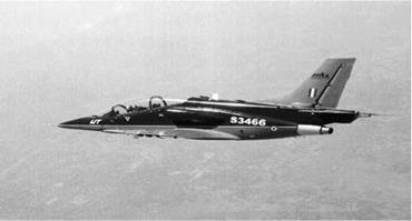
HJT-36 (Figure A13) is an Intermediate Jet Trainer (IJT) aircraft under development by Hindustan Aeronautics Limited (HAL) for the Indian Air Force. It is slated to replace the aging HJT-16 Kiran aircraft, which is currently used by the Indian Air Force. It has a conventional jet trainer design, with a low, swept wing, staggered cockpits, and small air intakes on either side of its fuselage. It has manually operated flight controls with three-axes trim capability using electrical actuators. With an overall length of 11.0 m, a service ceiling of 9 km, and a
|
|
|
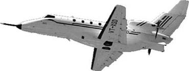
FIGURE A14 HANSA two-seater aircraft. |
maximum takeoff weight of 4500 kg, the aircraft can achieve a maximum Mach number of 0.75.
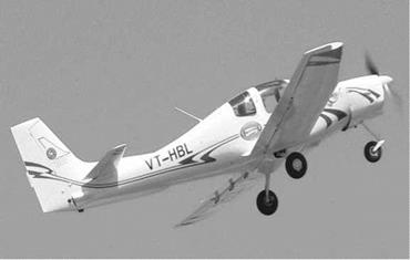
HANSA-3 aircraft (Figure A14), designed by National Aerospace Laboratories of India, is an all-composite light trainer aircraft ideal for training, sport, and hobbyflying. It is certified under FAR-23 and is successfully flying in various flying clubs of India. Its main features include a neat cockpit with good visibility, dual controls, and turbo charged engines with a constant speed propeller. It has an overall length of
7.6 m, wing span of 10.47 m, and all-up weight of 750 kg with usable fuel capacity of 85 L. It has a maximum cruise speed of 96 knots.
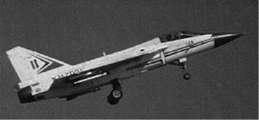
Aircraft Tejas (Light Combat Aircraft – LCA; Figure A15) is designed and developed by Aeronautical Development Agency (ADA), India, with an aim to replace the aging MiG-21 aircraft as the Indian Air Force’s primary multirole tactical aircraft. It is a single engine tail-less delta wing aircraft designed to be aerodynamically unstable in the longitudinal axis. The wing supports three-segment leading edge slats
|
|
and two-segment elevons that span the entire length of the trailing edge. The elevons are the primary control surfaces in pitch and roll. In order to stabilize the airframe and achieve the desired performance over the entire flight envelope, it incorporates a quad redundant full authority fly by wire (FBW) flight-control system (FCS). Its takeoff weight is around 8500 kg and has a maximum speed of 1.8 Mach.
Aircraft have several instruments that aid the pilot in flying. These can be categorized according to their use, e. g., flight instruments, engine instruments, navigational instruments, environmental instruments, electrical system instruments, and so on. Some of the instruments that fall in the category of flight instruments are discussed in Refs. [1,11]. Sensors/transducers are used to measure control positions, pressures, temperatures, and loads. The electrical signal from each transducer is routed through an instrumentation wiring to a signal conditioning circuit or device in the airplane. The signal conditioning would include multiplexing, commutating, digitizing,
ADC/DAC conversions, time-code generation, and pulse code modulation. Optical head-up display allows the pilot to observe the flight instrument information presented in the head-up form as well as the out-of-window view of the world.
Air Data Instruments: These instruments use a pitot-static system to measure ambient atmospheric pressure. Ambient or static pressure is measured through a set of holes provided on the side of a tube projecting into the free stream, typically on both sides of the fuselage (see Figure A1). To minimize the errors in the measured static pressure, the sensor is placed clear of the disturbed airflow. The pitot or the total pressure is sensed by the open end of the pitot-static tube, which is directly facing the oncoming airflow. The pitot pressure is the sum of static and dynamic pressures, the latter caused by the forward movement of the aircraft. Nose boom allows measurements of pressure and flow angles far in front of the fuselage. For flow angles the differential pressures are measured in both the axes: horizontal and vertical relative to the aircraft. These differential pressures along with the dynamic pressure (at the aircraft nose boom) are used and the flow angles are computed. In many situations five-hole probes are employed to measure 3-D flows. These probes can determine pitch and yaw angles also. Interestingly, a simple relation exists between yaw coefficient and measured pressures: Cyaw = PPl_Pp> . . From this coefficient yaw angle can be computed. However, in reality algorithms to accurately compute various such quantities would be complicated.
Pressure Altimeter: This is used to measure the aircraft altitude. It is basically a pressure transducer calibrated to read height above a specific pressure datum. It measures ambient pressure and indicates the value of the altitude on the instrument dial. The altimeter readings can become inaccurate at higher altitudes where the pressure change with a change in height is small.
Air Speed Indicator: The air speed indicator measures the dynamic pressure, which is computed as the difference between the pitot (total) and static pressure and converts it to airspeed. As the airspeed indicator is usually calibrated to standard sea – level conditions, the speed indicated is called IAS. The IAS corrected for the instrumentation errors and compressibility effects gives the EAS. The TAS can be obtained from the EAS by accounting for the change in the air density from standard sea-level conditions (see Equation A.11). The compressibility and density corrections are normally included in the navigation computer from which CAS and TAS can be found.
Mach Meter: This instrument comprises both the pressure altimeter and the air speed indicator. Mach number is defined as the ratio of TAS to local speed of sound (see Section A1). In Mach meter, the altimeter and ASI capsules are linked to the pointer of the Mach meter through links and gears. The pointer rotates on a dial indicating the airspeed in terms of Mach number.
Vertical Speed Indicator: This is also known as the rate of climb/descent indicator. It indicates the rate of change of height per minute as the aircraft is climbing or descending. It essentially senses the pressure difference between the pressure in the instrument casing and the static pressure inside the capsule, due to a change in height. The capsule is connected to a pointer, which moves on the dial. In level flight, the pressure in the instrument casing is equal to the static pressure in the capsule and the pointer will indicate zero.
|
FIGURE A12 SARAS transport aircraft. |
A few important aspects of flight vehicle performance are mentioned here.
The drag force acting an aircraft is typically a function of the lift coefficient and Mach number.
|
Cd = f (Cl, M) |
|
The equation for aircraft drag polar, given by Equation A.22, can be expressed as Cd = CDo + KC2l (A.38) where K can be estimated from flight data using parameter-estimation techniques. The theoretical value for the drag-due-to-lift factor K at subsonic speeds is given by 1/pAe, while its value at transonic and supersonic speeds is close to 1/Cl. Assuming thrust T to be inclined at angle sT with the flight path direction, the equations of motion for a level (U = 0) unaccelerated flight can be expressed as |
|
T cos sT = D T sin sT + L = W |
|
(A.39) |
|
For small values of sT, Equation A.39 becomes |
|
T = D L=W |
|
(A.40) |
|
Rearranging Equation A.40, the required thrust for an unaccelerated level flight is given by |
|
W |
|
(A.41) |
|
L/D |
|
Thus, minimum thrust is required where L/D is maximum. If V is the velocity of the aircraft during level unaccelerated flight, and the lift is equal to weight, we have |
|
I 2W VpScL |
|
/2W3c2 V pSC3l |
|
(A.42) |
|
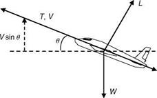
FIGURE A11 Airplane in a steady climb. |
Another important parameter in aircraft performance is the rate of climb. Compared to the level unaccelerated flight, the thrust in this case, in addition to overcoming drag, will also be required to compensate for the component of weight (Figure A11).
T = D + W sin U
The vertical velocity component gives the rate of climb, as shown in Figure A11.
Rate of climb = V sin U
The topic of performance is incomplete without the mention of engines used for propulsion. The piston engines with propellers still rule the roost in low-speed flights while gas turbine engines are used for jet propulsion at higher speeds. Turbo jets are equipped with a compressor, a combustion chamber, turbine, and exhaust nozzle. Thrust is provided by reaction of the exhaust gases thrown backward through the nozzle. Another type is the turbofan or the bypass engine, which has a large fan that accelerates the air ahead of the compressor, thus resulting in more thrust with higher efficiency. While turbojet and turbofan engines have rotating parts, there is another type called the ramjet, which uses the ram effect generated from the forward speed to pass the compressed air to the combustion chamber and out of the exhaust nozzle at very high speeds. As is obvious, ramjet will give no thrust at zero forward speeds.
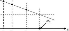
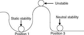
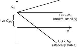
Neutral and maneuver points are important longitudinal stability parameters, which critically determine the aft CG limit of an aircraft. Since these parameters are a function of speed, AOA, external store configuration, control surface deployment (slats), etc., extensive flight tests are conducted to accurately determine these critical stability parameters. Existing methods based on steady-state trim flights turn out to be time-consuming and are error-prone because the results are dependent on air data and aircraft weight. An alternative approach, based on system theoretic concepts, is to estimate aircraft longitudinal static and dynamic stability from flight dynamic maneuvers in terms of neutral and maneuver points. In this procedure, the stability information is extracted from the short-period dynamic response of the aircraft, which leads to substantial reduction in flight test time compared with the conventional steady-state flight tests. Since this method does not use air data information or mass/inertia data, the resulting estimates of neutral and maneuver points are generally more accurate [9]. The neutral point is related to short-period static stability parameter Ma and hence the natural frequency (see Chapter 4). We estimate Ma values (using the parameter-estimation method) from short-period maneuver flight data of an aircraft, flying it for different CG positions (minimum three), and then plot with respect to CG, and extend this line to the x-axis. The point on the x-axis when this line passes through ‘‘zero’’ on the y-axis is the neutral point (see Figure A10). The distance between the neutral point NP and the actual CG position is called the static margin and when this margin is zero, the aircraft has neutral stability.
![]()

![]()
![]()
![]()
![]()
 Ma
Ma
|
 (A.37)