Category Helicopter Performance, Stability, and Control

The Lift on a Blade Element

The momentum method gives much insight into conditions at the rotor and in the wake, but it does not deal with the actual development of thrust—that is, the lift on the individual blade elements. The mechanism by which lift is developed by an airfoil is explained in textbooks on airplane aerodynamics, and that explanation applies just as well to an element of a rotor blade as to a section of a wing.

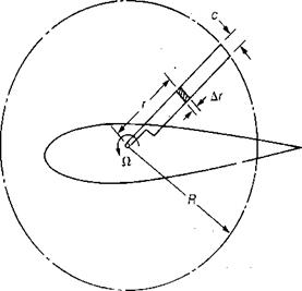
The geometry of a blade element is shown in Figure 1.5. A blade element is one small portion of the blade a distance, r, from the center of rotation with a spanwise dimension, Ar. The increment of lift, AL, on this blade element is:

AL = q СісАг

The local dynamic pressure, q, is a function of the velocity due to rotation at the blade element. This velocity is zero at the center of rotation and increases linearly to the tip. To express this velocity, it is convenient to use the rotational speed in terms of radians per second, ft. The local velocity at the blade element, V/} is:

V{= ftr ft/sec

At the tip, the tip speed, VT, is:

FT = ClR ft/sec

Tip speeds on modern helicopters are selected to be as high as they can be without encountering compressibility effects on the advancing blade in forward flight. These effects will be discussed in more detail in Chapter 3. At this point, it is enough to state that design tip speeds on both the main and tail rotors fall in the region between 500 and 800 ft/sec. Since tip speeds fall into this rather narrow band, it is usually more convenient in studying rotor aerodynamics to use this as a parameter to measure rotor speed rather than rpm, which will vary widely with rotor size. Note that

The local dynamic pressure, q, at the blade element is:

y = {p(Clr)2

The local lift coefficient, ch may be written as:

Ci = a a

where a is the local angle of attack in radians, and a is the slope of the lift curve per radian. Since the actual angle of attack including induced effects will be used, the correct lift curve slope is that corresponding to a two-dimensional airfoil. Con­ventional airfoils at low Mach numbers have lift curve slopes of approximately 0.10 per degree or 5.73 per radian. This value increases slightly with Mach number and will be assumed to be 6.0 for use in this type of simple rotor analysis.

The local angle of attack is determined by the geometric pitch of the blade, 0, and the local inflow angle, ф, as shown in Figure 1.6.

a = 0 – ф

The inflow angle, ф, is defined by the two mutually perpendicular velocities, fir and vly such that:

ф = сап"^

If ф is less than 10° — and it is for most of the rotor—then the small-angle assumption may be used:

ф = radians llr

FIGURE 1.6 Orientation of Blade Element and Local Velocities

Thus the local angle of attack is:

a = 0 — rad Пт-

and

ct = a I 0 —

The increment of lift on the blade element is:

AL = – (Пг)2<г f 0 — j cAr

The actual power is the induced power divided by the Figure of Merit:

I D. L.

, _ h’.p_ T J 2p

‘P’“ F. M. 550 (F. M.)

At sea level, this becomes:

Ту/РЇ.

■p’act 38 (F. M.)

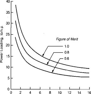
The power loading in pounds per horsepower can be obtained by rearranging the equation:

T 38 (F. M.)

h-p-aa y/D. L.

A plot of this equation is presented in Figure 1.4 for Figure of Merit values of 1.0, 0.8, and 0.6—corresponding to the ideal rotor, to a very good practical rotor, and to an average rotor respectively. (Note: A low Figure of Merit in hover does not necessarily represent a poorly designed rotor. More commonly, it represents a rotor that has been designed for high-speed flight and is not being operated at its optimum hovering conditions.) It may be seen from Figure 1.4 that high power loadings go with low disc loadings and high Figures of Merit. The use of this chart allows a first approximation to be made of the power required to hover. The example helicopter has a disc loading of 7.1 lb/ft2. If a Figure of Merit of 0.8 is assumed for its rotor, then the power loading is 11.4 lb/h. p. and, since the helicopter weighs 20,000 lb, the power required by the rotor is 1,760 hp. If the rotor radius had been 40 feet instead of 30, the disc loading would have been 4.0 lb/ft2, and the power required would have been only 1,320; but the tail boom would have had to be 10 feet longer to achieve clearance between main and tail rotors, and the nose would have had to be longer to balance the tail boom. As a

consequence, the reduction in power required would have been obtained at the expense of added structural weight and a larger overall size with, perhaps, little increase in payload capability. Making decisions on this type of trade-off represents much of the engineering effort during the early stages of the development of a new helicopter design.

The ideal power derived from momentum considerations is the power required by a rotor consisting only of an idealized actuator disc without regard for the drag of the actual blades. In this sense, the ideal power is analogous to the induced drag of an airplane wing and, as a matter of fact, is generally called induced power. The actual power, of course, is higher than the induced, or ideal, power. The ratio of induced power to actual power is known as the Figure of Merit (F. M.):

Induced power

F-M – = -7——— r-^——–

Actual power

It will later be shown that the value of the Figure of Merit is a function of the rotor geometry and of the rotor operating conditions. Whirl tower tests of conventional helicopter rotors have shown that the maximum Figure of Merit that can be expected in practice is 0.75 to 0.80.

The minimum—or ideal—power required to produce rotor thrust may be determined from momentum considerations as the energy per second dissipated at the rotor:

Er/scc = (Force) (Velocity) = T vx ft lb/sec

Since 550 ft lb/sec is the equivalent of one horsepower, the ideal power is:

or

h. p

At sea level, the ideal power is:

Ty/51.

38

From this equation, it may be seen that for a given rotor thrust, the higher the disc loading, the higher the power required. During the early days of helicopter development, when power plants were relatively heavy, designers minimized the power required by using low disc loadings of 2 to 3 lb/ft2. The introduction of lightweight turbine engines has made it possible to put less emphasis on low power requirements and more emphasis on designing compact helicopters with minimum structural weight. For this reason, over the years disc loadings have been increasing steadily until values of 10 to 12 lb/ft2 are considered feasible for helicopters that do not have to operate close to loose surfaces.

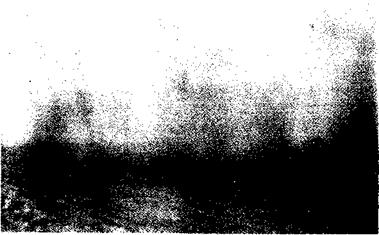
The induced velocity in the wake of a hovering helicopter can produce operational problems if the hovering is done close to dust, sand, snow, or other loose surfaces. The higher the disc loading, the stronger is the placer mining capability of the wake. Helicopter disc loadings range from 4 to 12 lb/ft2, and the corresponding downwash velocities in the remote wake range from 35 to 58 knots. Even the lower velocities can lift enough dust or snow to effectively cut off the pilot’s view of the ground, as is shown in Figure 1.2. At the higher disc loadings, gravel can be entrained in the wake and forced to circulate through the rotor and the engine intake.

A high rotor downwash velocity also makes it difficult to work under a hovering helicopter while hooking up a sling load or guiding the pilot to a precision landing.

Thus it may be seen that the higher the disc loading, the more severe are the operational problems. For nonhelicopter hovering aircraft that use very high disc­loading devices such as propellers or jet engines for lift, these problems become severe enough to limit landings and takeoffs to hard-surfaced, prepared areas. In light of these problems, one might ask: "Why use high disc loadings?” The answer is that high disc loadings permit design of compact helicopters with low empty weight, which for many applications are the most efficient aircraft.

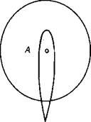
Another effect of the rotor-induced velocities in hover is to produce a download on the fuselage and any other aircraft components that are located under the rotor. The rotor wake contracts from the diameter of the rotor to its remote wake size in about a quarter of a rotor radius, as shown in Figure 1.3, which was obtained using smoke for flow visualization. For most helicopters, the fuselage can be considered to be immersed in the remote wake and to receive the full effect of the downwash. The download, or vertical drag, on the fuselage can be computed from the standard equation for drag:

D = CDqS

The dynamic pressure in the remote wake, q2), is equal to the disc loading of the rotor. This statement may be proved by using the relationships:

v 2 — 2vl = 2

and

Thus

or

q2 = D. L. lb/ft2

A first estimate of the download may be obtained by assuming an effective drag coefficient of 0.3 for all the aircraft components in the remote wake. (A more elegant procedure will be found in Chapter 4.) For this estimate, the vertical drag, Dyf is:

Dv= (0.3) (D. L.) (Projected area of all affected components)

It is often convenient to express the vertical drag as a fraction of the gross weight:

Dv (0.3)(D. L.)(Projected area)

G. W. = (D. L.)(Disc area)

or:

Dv 0.3(Projected area)

G. W. Disc area

The example helicopter has a projected area of 380 ft2 and a disc area of 2,827 ft2. It thus has a download of 4% of its gross weight. The rotor thrust required to support a hovering helicopter and its vertical drag is:

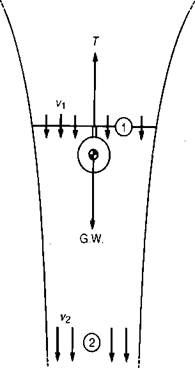
The elements of the thrust equation can be evaluated from a study of the flow field in Figure 1.1. In that figure, the three regions of interest have been numbered 0 for the region high above the rotor, 1 for the plane of the rotor, and 2 for the region far below the rotor in the fully developed rotor wake. The mass flow per second in the plane of the rotor is:

mjste = p vx A slugs/sec

where p is the density of the air in slugs/ft3, vx is the induced velocity, at the rotor plane, and A is the area of the rotor disc. The total change in velocity, Av, between region 0 and region 2 is:

Av = v2 — v0 ft/sec

Since far above the rotor the air has no velocity, the total change in velocity is:

Av = v2 ft/sec

Thus the expression for rotor thrust may be written:

T = p vxAv2 lb

The equation for thrust in this form is not very useful. Fortunately, a relationship between vx and v2 can be derived by equating the rate of energy dissipated at the rotor to the rate of energy imparted to the wake. Since the rotor and its wake make up a closed system, these two rates of energy must be equal. The energy per second dissipated by the rotor, Eg/sec, is:

Eg/sec = Force x Velocity

or

Eg/see = Tvx ft lb/sec

or

Eg/sec = pvA v2 ft lb/sec

The energy per second imparted to the wake, Ew/stc, is the total change in kinetic energy. Since there is no kinetic energy far above the rotor, the total change is the value found in the remote wake:

Ew/sec= і(/я2/sec) v

The mass flow per second in the remote wake, mjstc, is the same as the mass flow at the rotor, mjstc. This is a consequence of the Law of Continuity, which also applies to such things as syrup pouring from a pitcher. Once the flow is established, the amount of syrup reaching the pancake per second is the same as that leaving the lip of the pitcher even though the cross-section of the flow is larger at the top than at the bottom. The energy in the wake thus becomes:

That is, the induced velocity in the remote wake is twice the induced velocity at the rotor disc.

The equation for thrust becomes:

T=2pvA lb

and consequently the induced velocity in the plane of the rotor, vlt is:

The rotor thrust, T, divided by the disc area, A, is the disc loading, D. L., in pounds per square foot. The equation for the induced velocity may be written:

For sea-level standard conditions, the density, p, is 0.002377 slugs per cubic foot, so that:

= 29 y/Dl. ft/sec

Source: Hill, “A Promising Concept for the Joint Development of Military Intra-Theater and Commercial Inter-Urban VTOL Transports," 24th AHS Forum, 1968.

The example helicopter described in Appendix A has a design gross weight of 20,000 lb and a rotor radius of 30 ft. Assuming that the rotor thrust is equal to the gross weight, the disc loading is 7.1 lb/ft2, the velocity at the disc is 39 ft/sec, and the velocity in the remote wake is 78 ft/sec or 46 knots. For computations involving induced velocities produced by tandem-rotor helicopters in which one rotor overlaps the other, only the net projected area should be used in computing the disc loading. Similarly, with a coaxial helicopter, only the disc area of a single rotor should be used.

MOMENTUM METHOD

Basis of the Theory

Like any physical system, the hovering helicopter must obey the basic laws of physics. One of these laws was stated by Newton: "For every action, there is an equal and opposite reaction.” In the case of the helicopter in hovering flight, the action is the development of a rotor thrust equal to the gross weight. The reaction

In the subsequent text, there are a number of times when some light can be shed on the theory by using specific numerical examples. For this purpose, a typical helicopter has been defined and designated the example helicopter. The characteristics of this aircraft are listed in Appendix A.

®v0

is represented by the acceleration of a mass of air from a stagnant condition far above the rotor to a condition with a finite velocity in the wake below the rotor, as shown in Figure 1.1. The conditions at the rotor are governed by the familiar relationship:

Force = (Mass) (acceleration)

For systems such as rotors that are accelerating a mass of air on a continuous basis, the equation may be written as:

Rotor Thrust = (Mass flow per second) (total change in flow velocity)

or:

T = (яг/sec) (Д?)

The purpose of this book is to provide both the student and the practicing helicopter aerodynamicist with the information they need to analyze the performance of an existing helicopter or to participate in the design of a new helicopter. This text should also be helpful for those in the helicopter industry who work with aerodynamicists and may have been baffled by what seemed to be an art rather than a science. The information presented here includes the derivation of the theory behind the various methods of analysis, appropriate experimental data to correlate and supplement the theory, and charts that permit rapid analysis. A special attempt is made to relate helicopter aerodynamics to airplane aerodynamics for those who are making the transition.

To focus on the practical aspects of the subject, an "Example Helicopter” is defined in Appendix A and is consistently used throughout the book to illustrate, by numerical calculations, the application of the analysis. These calculations are listed at the end of each chapter, along with a listing of "How To’s,” which can be used to shorten the search for a specific subject. Although no problems are presented at the ends of chapters, they can easily be generated using the example helicopter calculations as examples and the helicopter parameters selected by the instructor or the student. The generation of problems involving extension of the theory, wherein the proof is left to the ambitious student, is left to the ambitious instructor.

The first six chapters are devoted to tfye various aspects of helicopter performance. Chapters 7, 8, and 9 cover stability and control. The final chapter presents the tradeoff considerations that the engineer must face during the

preliminary design phase to ensure both good performance and good flying qualities.

Aeroelastic rotor effects, including vibration, oscillating loads, and the stability of nonconventional rotors, are not addressed. For an understanding of these mysterious effects, other sources must be consulted.

The material includes almost all of the information and methods that I have found to be significant as a working aerodynamicist for Hughes, Sikorsky, Bell, and Lockheed since 1952. The outline of the book was first developed as lecture notes used in teaching engineering extension courses at the University of California at Los Angeles.