Category Model Aircraft Aerodynamics

Laminar flow causes considerably less skin friction than turbulent In a laminar boundary layer the air moves in very smooth fashion, as if each tiny layer of the fluid was a separate sheet or lamina, sliding past the others with only slight stickiness or viscous stress between. There is no movement of particles of air up or down from layer to layer. The lowest lamina is stuck to the surface. The layer above it slides smoothly over this immobile layer, and the next above smoothly over that and so on until at the outermost limit of the boundary layer, the last lamina of all is moving almost at the speed of the main stream. The total thickness of the whole boundary layer may be a few hundredths of a centimetre. If measurements are made of the speed of flow at each level within this layer, diagrams such as Figure 3.1 may be drawn. Each arrow represents the flow speed at a point above the surface. It is found that the velocity increases fairly steadily from bottom to top. The laminae near the surface are creeping along, those next above move only slightly faster. It is this slow, smooth movement of the layers near the surface that reduces the skin friction. But because these layers are so slow, and receive little traction fri>m the main stream, they are all too easily brought to a standstill.

Reynolds number applied to a wing chord is not the same as the Re inside the boundary layer itself. As the airflow meets the wing near the leading edge, there is a point, called the stagnation point (Fig. 2.2) where the flow divides, some to pass above and some below the wing. The Re in the boundary layer at this point is zero, since the distance covered over the surface is nil. The boundary layer flow moves from the stagnation point along the skin of the wing and the Reynolds number at each point is based on the distance of that point measured round the aerofoil profile, from the stagnation point Hence the Re in the boundary layer increases as the distance from the stagnation point increases.

By the time the boundary layer reaches the trailing edge its Re will be higher, because of the greater distance covered, than the average worked out crudely using the wing chord, which is the straight line distance from leading edge to trailing edge. Since most aerofoils have different contours on upper and lower surfaces, and the wing is normally operating at some angle of attack, the boundary layer Re at opposite stations on top and bottom will differ a little. In what follows it is important to distinguish the so-called ‘critical Re’ of an aerofoil profile from the ‘critical Re’ in the boundary layer itself.

Experimental work published by Osborne Reynolds in 1883 showed that there are two distinct types of flow, laminar and turbulent. These may change from one to the other according to particular conditions. Which type of flow prevails in the boundary layer at any point depends on the form, waviness and roughness of the surface, the speed of the mainstream measured at a distance from the surface itself, the distance over which the flow has passed on the surface, and the ratio of density to viscosity of the fluid. A variation in any Of these factors can bring about a change in the boundary layer. Reynolds combined them all except surface condition, into one figure, the Reynolds number. The formula for Reynolds number is:

Reynolds Number, Re = Viscosity x Velocity x Length

, , . . , , „ « „ , pVL V x L

In the standard symbols: Re = x V x L or—————— or———-

Ц ft v

(The Greek letter v ‘nu’ stands here for the kinematic viscosity of the fluid)

Viscosity is measured in kilogrammes per metre per second, the standard value for air is 17.894 x 10-6 or.0000179 kg/m/sec (.373 X 10-6 slugs/fl/sec). As the equation shows, as viscosity increases, Reynolds number decreases. The average Re of a model wing or tail surface may be found using the normal flying speed as the velocity and the average chord as the length, so, for example, a wing of chord 0.1 metres flying at 10 metres per second with standard density and viscosity has Re (1.225/.000017894) x 0.1 x 10 = (68459) x 1 — 68459. A useful abbreviation for most modelling needs is thus provided by the simplified equation:

Re = 68459 x VL

where V and L are in m/sec and metres. If V and L are in ft/sec and feet, Re = 6363 x VL. As density, velocity and length increase, Reynolds number increases. It is often suggested that since density and viscosity are not under control, for modelling purposes the VL figure alone is important and in most ways this is true providing it is remembered that the VL is expressed in units (metres x metres/sec., or ft x ft/sec.) whereas the Re is non – dimensional. For a fuller understanding of Re effects, however, the ratio of inertia forces to viscosity forces in the boundary layer is what counts, relative to the speed of flow at each point This ratio (toes vary appreciably according to seasonal conditions and altitude. Reynolds numbers rise in winter. (See Appendix 1).

3.2 TYPICAL AVERAGE REYNOLDS NUMBERS

Aircraft type

Commercial aircraft Light aeroplane

Sailplane at max. speed, wing root Sailplane at min. speed, wing tip

Pylon racing model aeroplane at max. speed

Hang gliders, man-powered aircraft, ultra light aeroplanes

Multi-task R. C. sailplanes in speed task: when soaring:

Large model sailplanes Thermal soaring: penetrating:

A-l, A-2 sailplanes, Wakefields, Coupe d’Hiver etc. max.

min.

Indoor models, ‘peanut’ scale etc.

Large soaring bird, (e. g. albatross or eagle) Seagull

Butterfly (gliding) 7,000

(The above figures are all approximate and depend on the actual speeds of flight, wing chords, etc.)

Typical values of Re for various types of model are shown in the table. It is important to remember that the chord of a wing tip is usually smaller than the root, so the Re is less. For the example model with Re average about 68000, the tip chord might be 0.08 metres and the root 0.12, so the Re at each would be about 48000 and 81000. This is of special importance for the phenomenon of wing tip stalling in models.

No model flies at constant speed for long. Each change of speed alters the Re, in simple proportion. The faster the flight, the higher the Reynolds number. If the tailplane has smaller chord than the wing, the operating Re will be less for the tail.

3.1 THE BOUNDARY LAYER

The most important differences between model and full-sized aircraft aerodynamics can be attributed to the boundary layer, the thin layer of air close to the surface of a wing or any solid body over which the air flows. Two properties of air, its mass and its viscosity, determine the behaviour of the boundary layer. Viscosity may be roughly described as the stickiness of any fluid. Treacle and glycerine are highly viscous at normal temperatures. Cream and water are less viscous, air and other gases are less viscous still. The viscosity, like the density of air, is beyond control for practical purposes in model aerodynamics. Like air density, it does vary with temperature and air pressure, as Lnenicka’s chart in Appendix 1 shows. Inertia opposes change of direction or velocity. Viscosity resists shearing flows and tends to keep the fluid in contact with surfaces. In situations where fluid in the boundary layer over a surface is accelerating or decelerating, forces arising from mass and from viscosity interact, sometimes reinforcing one another, sometimes in mutual opposition. Where velocities of flow are high and the curvature of surfaces relatively large in radius, as with full-sized wings at high speeds, mass inertia is dominant, the effects of viscosity, though not negligible, are smaller. With model wings, at low speeds, viscous forces become relatively much more important A very small wing, such as that of an insect, operates in a fluid which seems relatively much more viscous than the air does to the wing of an airliner. Model aircraft, and full-sized sailplanes, man-powered aircraft, hang-gliders, etc., come somewhere between. It cannot be expected that a model wing, even one made to exact scale from a full-sized prototype, will behave in exactly the same way as its larger counterpart Unfortunately such scale effects almost invariably work to the disadvantage of the smaller aircraft.

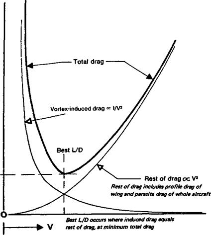
The total drag of the aircraft is composed of the total vortex and all other drags at each speed. Where the vortex drag equals all the rest, i. e., where the two lower curves in Figure 2.11 intersect, drag is a minimum for the whole aircraft Since lift is constant for a given mass of aircraft in level flight it is at the minimum drag point on the curve that the best L/D ratio of the aircraft occurs. Another, slightly more elaborate, presentation of this information appears in Figure 4.10, and in Figure 4.4 the shape of the polar curve of a sailplane is directly related to this same curve, although presented in different form in that figure, as sinking speed plotted against velocity rather than total drag against Cl.

In Figures 2.8-10 Де types of drag are illustrated. Induced drag is now called vortex drag because it is associated whh the rotating vortices which trail behind any wing, or any surface, which is yielding aerodynamic lift The appearance of Де vortices is directly associated wiffi the lift Де higher Де lift coefficient of a given wing. Де more significant is Де effect of Де vortices. Since when flight speed, V, is low, a given model must work at a higher lift coefficient Дап when V is high, Де induced drag increases as the velocity decreases. (Maffiematically, vortex-induced drag is proportional to L/V2.) This is the major, though not Де only cause of Де reduction of L/D at low speeds mentioned above.

Fig. 2.10 Skin friction or viscous drag

smooth wave-free skin _

Low drag surface

High drag, surface

2.IS PROFILE DRAG

Form or pressure drag is caused by the total of all the pressure variations over a body as the air flows round it, and skin friction or viscous drag is caused by the contact of the air with the model’s surfaces. Although it is useful to separate these different types of drag for purposes of study, it is clear that they almost always occur together. For instance, the wings shown in Figure 2.8 will produce both form drag and skin friction in addition to vortex drag. The body whose skin is sketched in Fig. 2.10 will probably be part of wing or fuselage which has form drag also. The relationship between skin drag and form drag is particularly close: the two affect one another. For example, skin friction is very much governed by the speed of the air flow, and the speed of the local flow next to the skin is

mainly determined by the shape of the body as a whole. (See Bernoulli’s theorem, Chapter 3.) For this reason, particularly when wings are concerned, skin friction and form drag are commonly taken together and termed profile drag. In contrast to induced drag, skin friction and form drag are both directly proportional to V2. Thus, as the induced drag falls with rising speed, the form drag and skin drag rise, and vice versa. The result, in graphical form, is shown in Figure 2.11.

All parts of a model, including wings, tail fuselage and every component exposed to the air flow, contribute drag. Even the insides of cowlings, wheel fairings, etc., will add some drag if air passes through them. As with lift, the actual drag force generated depends on flight velocity, air density, size and shape of the model. The drag coefficient, like the lift coefficient, sums up all the features of the model and is a measure of its aerodynamic ‘cleanliness’. The formula is of the same type as that for lift:

DRAG = D = V4xpxV2xSxCD

The S, or area in this formula is normally the wing area of the whole aircraft. If the total surface area is used (including tail) for the Cl, the same total area must be used for the drag equation. This enables the drag and lift forces to be compared, usually in the form of

V+’kp V* = constant

Fig. 2.7 The venturi

a ratio, the lift to drag ratio or L/D. For level flight, lift will equal weight, which is constant (ignoring fuel consumption). Thrust can be increased or decreased by variations of throttle setting. This will change the drag force, since for level flight in equilibrium, thrust and drag are equal. At high speed, thrust is large and drag is large, but the total lift force remains the same, equal to the weight The ratio of lift to drag is low; drag has increased because of the high speed. At low speeds, still maintaining level flight, drag

Fig. 2.9 Form or pressure drag

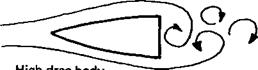High drag body

27

reduces up to a point while lift still equals weight. Hence the L/D ratio increases. This improvement in drag force does not continue down to the slowest speed for any given model, since, as will appear, the total drag coefficient itself begins to increase rapidly at low speeds, and this is enough to outweigh the reduction in V. Hence at some speed the model achieves its maximum L/D ratio. The value of this ratio gives a rough measure of the all-round efficiency of the model.

As with lift, confusion arises if wind tunnel tests are wrongly interpreted. In tests of isolated bodies such as fuselages, wheels, etc., Де measure of size, S, used in the drag formula is Де cross sectional area of the object tested. This gives a wholly ffifferent result from Де drag coefficient of such items when Деу are related to Де wing area of a whole aircraft Whh wing drag figures from tunnel tests, Де same applies as to section lift coefficients. The real wing in flight does not reproduce Де test figures across Де whole span. It is hardly ever necessary to calculate the actual drag of model components. The main toing is to know how drag is caused and how to reduce it. Modellers quite often speak of increasing lift by changing Де trim or using a different wing section. In level flight the lift force equals Де weight and Дів remains true after Де trim or aerofoil change just as before. Hence akhough Де lift coefficient, Cl, may have been increased, Де lift force remains equal to Де weight in level flight. Every change of this kind however, does change Де drag of Де aircraft If the drag is regarded as Де inevitable price paid for keeping a given model in Де air, reducing the drag price always makes for a more efficient flight

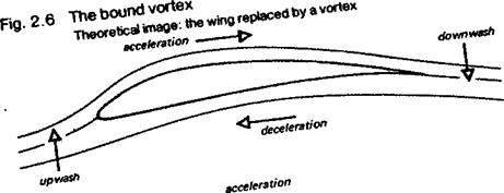
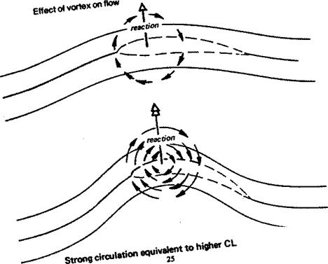
The upwash ahead and downwash behind a wing, with the accelerations and decelerations above and below, suggest that a diagram like that in Figure 2.6 may be drawn. The streamlines behave as if, instead of a wing, there was a rotating and moving cylinder of air, a vortex, with its axis aligned with the wing. Such a cylinder would cause upwash and downwash, acceleration and deceleration of flow, in very much the same way as a real wing, and it would cause identical reaction forces. The strength or speed of the vortex circulation would determine how much reactive force was produced. Many experiments have shown that rotating cylinders do produce lift, but the main value of this idea is that it enables the lifting ability of any wing to be explained or calculated in terms of the strength of circulation of the imaginary vortex. The rotating cylinder is termed the bound vortex because it is supposed to be tied to the wing and moves along with it. The idea of the bound vortex is particularly useful in calculations of the lift distribution spanwise across real wings. The strength of the bound vortex at each point is a measure of the lift at that location. The concept is a mathematical model rather than a physical reality.

2.5 BERNOULLI’S THEOREM

Bernoulli’s theorem connects the pressure measured at any point in a fluid such as air to the mass density and velocity of flow. This theorem is a special application of the laws of motion and energy which is of fundamental importance to aerodynamics and flight, as well as to liquid flows in pipes, channels and around the hulls of ships, etc.

If a small particle or cylinder of air is imagined as part of a general flow moving smoothly, or in ‘streamlineid’ fashion, the particle will be in equilibrium if the pressures acting on it from all directions are equal. If there is a pressure difference in any sense, the particle will accelerate or decelerate in accordance with the second law of motion. V, velocity, will increase if the pressure on the front face of the cylinder is less than that behind, V will decrease if the pressure behind is less than in front. Hence the particle will speed up as it approaches a region of low pressure, and slow down on approaching a high pressure zone. Since it is not isolated, but part of a general streamlined flow, the same laws apply to every particle in the flow, which therefore speeds up and slows down on approaching low and high pressure regions respectively. The simple mathematical expression of this principle is, where P stands for pressure:

P + VipV2 = Constant (Bernoulli’s theorem)

Air flowing at speeds of interest to modellers is constant in density. Pressure and velocity are the only variables; if one increases the other decreases under all circumstances. A well known application of the principle is the ‘venturi’ tube which is used in aviation to measure airspeeds or drive instruments, and in every day life to produce high speed jets from garden hoses, taps, etc.

A fluid passing through a constricted tube such as the venturi sketched in Fig. 2.7 contains no vacant cavities. The same mass of fluid must leave the exit, in each time unit, as the mass entering. In the constricted part of the tube, since the cross sectional area is small, the velocity of flow must increase to get the same mass through in the time available. This increase of velocity, in accordance with Bernoulli’s theorem, produces a reduction in pressure in the throat. The small cylinder of air imagined above becomes elongated and narrower in cross section in the throat, then returns to its original form after reaching the wider part of the tube. The ‘streamlines’ thus appear as shown.

A fluid passing over any body, so long as streamlined flow persists, will experience similar deformations of flow, with accordant velocity and pressure changes. This is particularly relevant to the flow over a wing.

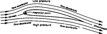
The Figure 2.2 showed, in accordance with Bernoulli’s theorem that when air passes over a wing it accelerates into the low pressure region on the upper surface. Somewhere it reaches the point of least pressure. From there onwards it flows towards the trailing edge against a pressure gradient tending to slow it down. The pressure above the wing behind the minimum pressure point, although it is increasing, is still lower than the normal or ‘static’ pressure of the main flow far away from the wing. On the underside, although the pressure is high on average, there is deceleration up to the maximum pressure point (which is often very close to the leading edge) and acceleration thereafter.

Further difficulty is caused by the tailplane’s contribution to the aircraft Cl – In modelling for competition purposes, the tail area and wing area are both taken into account to prevent competitors from trying to gain unfair advantage in wing loading by fitting oversized tailplanes. (That there is any advantage is an illusion, but the rule was intro­duced long ago and is unlikely to be changed in the F. A.I. Sporting Code. Any area added to the stabiliser has to be taken away from the mainplane.) If the tail or canard forewing does contribute some lift to the total, the Cl of the whole model may be determined using the combined areas in the lift formula. In full-sized aeronautics die aircraft Cl is usually determined in terms of the wing area alone. This is a convention, no more. Various other conventions are adopted about the parts of wings and tails that are (geometrically) inside fuselages, or enclosed by engine nacelles, etc. What area is actually used in calculations is to some degree a matter of choice and convenience. Problems arise only if inconsistent conventions are adopted.

2.4 STREAMLINED FLOW

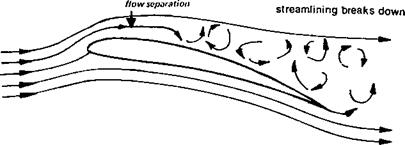
When the air meets any body, such as a wing, it is deflected over the surfaces. In accordance with Bernoulli’s theorem (see 2.12 below) above and below a wing there is a complex variation of velocity and pressure. For positive reaction, which is the basis of lift, there must be a positive difference in total pressures on top and bottom surfaces. The air over the upper surface is therefore made to flow over a longer route, so that it moves faster than that talcing a shorter route below. These effects are felt both ahead of and behind the wing. The flow ahead tends to be drawn upwards towards the low pressure region, which creates an upwash, and beyond the trailing edge it tends to return to its former position, so there is a corresponding downwash (Fig. 2.2). The pressure difference between the two surfaces may be increased up to a point by increasing the angle of attack, or increasing the camber or both. There is a very definite limit to this. If either the angle of attack or the camber is increased too much, the streamlining breaks down and the flow separates from the wing. This is explained in greater detail in Chapter 3. Flow separation not only creates a great deal of drag, but also changes markedly the pressure difference between upper and lower surfaces. The lift force is drastically reduced, the wing is stalled (Fig. 2.3).

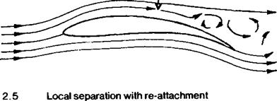
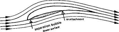
Flow separation on a smaller scale is common. On the upper surface, flow may separate somewhere before the trailing edge, as sketched in Figure 2.4, or, as suggested in

The importance of weight relative to wing area is apparent from the above. The wing loading, often written W/S and expressed in kilogrammes per square metre (pounds or ounces per sq. ft.), is the easiest way of portraying this relationship. The weight of a model, neglecting small changes caused by fuel consumption, is constant during one flight. The speed at a given trim (angle of attack) will depend entirely on the wing loading. This may be shown by re-arranging the lift formula to bring L/S onto one side. (L *= W in level flight.) Dividing both sides of the equation by S gives:

W/S = L/S = YipV^Cb

For gliders, and descending power models, lift and weight are not quite equal (Lift = WCos a, see Fig. 1.4) but for normal angles of dive or climb less than ten degrees there is very little difference and the wing loading formula holds good. Adding weight increases forward speed, but requires more power to sustain flight (In a glider a more powerful upcurrent is then needed for soaring.)

2.3 WING CL AND SECTION q

The Cl of a whole model or whole wing should not be confused with the lift coefficient determined in a wind tunnel for an aerofoil section. The section lift coefficient is sometimes written ci, in lower case letters, or Cl, to distinguish it but this is not always done and confusion results. The Cl of a real wing or tailplane cannot as a rule be arrived at by a simple transfer of values from a tunnel test of ci. The various effects of cross flow and downwash on a real wing cause the section lift coefficient to vary from place to place across the span, even if the wing is nominally at the same geometric angle of attack to the line of flight. The Cl finally arrived at is approximately the average of all the local values.