Category THEORETICAL AERODYNAMICS

The following are the three important concepts for visualizing or describing flow fields:

• The concept of pathline.

• The concept of streakline.

• The concept of streamline.

Pathline

Pathline may be defined as a line in the flow field describing the trajectory of a given fluid particle. From the Lagrangian view point, namely, a closed system with a fixed identifiable quantity of mass, the independent variables are the initial position, with which each particle is identified, and the time. Hence, the locus of the same particle over a time period from t0 to tn is called the pathline.

Streakline

Streakline may be defined as the instantaneous loci of all the fluid elements that have passed the point of injection at some earlier time. Consider a continuous tracer injection at a fixed point Q in space. The connection of all elements passing through the point Q over a period of time is called the streakline.

Streamlines

Streamlines are imaginary lines, in a fluid flow, drawn in such a manner that the flow velocity is always tangential to it. Flows are usually depicted graphically with the aid of streamlines. These are imaginary lines in the flow field such that the velocity at all points on these lines are always tangential. Streamlines proceeding through the periphery of an infinitesimal area at some instant of time t will form a tube called streamtube, which is useful in the study of fluid flow.

From the Eulerian viewpoint, an open system with constant control volume, all flow properties are functions of a fixed point in space and time, if the process is transient. The flow direction of various particles at time t forms streamline. The pathline, streamline and streakline are different in general but coincide in a steady flow.

Timelines

In modern fluid flow analysis, yet another graphical representation, namely timeline, is used. When a pulse input is periodically imposed on a line of tracer source placed normal to a flow, a change in the flow profile can be observed. The tracer image is generally termed timeline. Timelines are often generated in the flow field to aid the understanding of flow behavior such as the velocity and velocity gradient.

From the above mentioned graphical descriptions, it can be inferred that:

• There can be no flow through the lateral surface of the streamtube.

• An infinite number of adjacent streamtubes arranged to form a finite cross-section is often called a bundle of streamtubes.

• Streamtube is a Eulerian (or field) concept.

• Pathline is a Lagrangian (or particle) concept.

• For steady flows, the pathline, streamline and streakline are identical.

The rate of change of properties measured by probes at fixed locations are referred to as local rates of change, and the rate of change of properties experienced by a material particle is termed the material or substantive rates of change.

The local rate of change of a property r is denoted by dr(x, t)/dt, where it is understood that x is held constant. The material rate of change of property r shall be denoted by Dr/Dt. If r is the velocity V, then DV/Dt is the rate of change of velocity for a fluid particle and thus is the acceleration that the fluid particle experiences. On the other hand, dV/dt is just a local rate of change of velocity recorded by a stationary probe. In other words, DV/Dt is the particle or material acceleration and dV/dt is the local acceleration.

For a fluid flowing with a uniform velocity Vx, it is possible to write the relation between the local and material rates of change of property r as:

dr Dr dr dt = Dt – a?

Thus, the local rate of change of r is due to the following two effects:

1. Due to the change of property of each particle with time.

2. Due to the combined effect of the spatial gradient of that property and the motion of the fluid.

When a spatial gradient exists, the fluid motion brings different particles with different values of r to the probe, thereby modifying the rate of change sensed by the probe. This effect is termed convection effect. Therefore, Vx (dr/dx) is referred to as the convective rate of change of r. Even though Equation (2.17) has been obtained with uniform velocity Vx, note that in the limit St ^ 0 it is only the local velocity V which enters into the analysis and Equation (2.17) becomes:

dr Dr dr

dt Dt dx

Equation (2.18) can be generalized for a three-dimensional space as:

where V is the gradient operator (= id/dx + jd/dy + kd/dz) and (V ■ V) is a scalar product (= Vx d/dx + Vy d/dy + Vz d/dz). Equation (2.19) is usually written as:

(2.20)

when n is the velocity of a fluid particle, DV/Dt gives acceleration of the fluid particle and the resultant equation is:

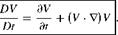(2.21)

Equation (2.21) is known as Euler’s acceleration formula.

Note that the Euler’s acceleration formula is essentially the link between the Lagrangian and Eulerian descriptions of fluid flow.

Basically two treatments are followed for fluid flow analysis. They are the Lagrangian and Eulerian descriptions. Lagrangian method describes the motion of each particle of the flow field in a separate and discrete manner. For example, the velocity of the nth particle of an aggregate of particles, moving in space, can be specified by the scalar equations:

where Vx, Vy, Vz are the velocity components in x-, y-, z-directions, respectively. They are independent of the space coordinates, and are functions of time only. Usually, the particles are denoted by the space point they occupy at some initial time t0. Thus, T(x0, t) refers to the temperature at time t of a particle which was at location x0 at time t0.

This approach of identifying material points, and following them along is also termed the particle or material description. This approach is usually preferred in the description of low-density flow fields (also called rarefied flows), in describing the motion of moving solids, such as a projectile and so on. However, for a deformable system like a continuum fluid, there are infinite number of fluid elements whose motion has to be described, the Lagrangian approach becomes unmanageable. For such cases, we
can employ spatial coordinates to help to identify particles in a flow. The velocity of all particles in a flow field, therefore, can be expressed in the following manner:

Vx = f (x, y,z, t) (2.15a)

Vy = g(x, y,z, t) (2.2)

Vz = h(x, y,z, t). (2.15c)

This is called the Eulerian or field approach. If properties and flow characteristics at each position in space remain invariant with time, the flow is called steady Bow. A time dependent flow is referred to as unsteady Bow. The steady flow velocity field would then be given as:

Liquids behave as if their free surfaces were perfectly flexible membranes having a constant tension a per unit width. This tension is called the surface tension. It is important to note that this is neither a force nor a stress but a force per unit length. The value of surface tension depends on:

• the nature of the fluid;

• the nature of the surface of the substance with which it is in contact;

• the temperature and pressure.

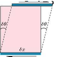
Consider a plane material membrane, possessing the property of constant tension a per unit length. Let the membrane have a straight edge of length l. The force required to hold the edge stationary is:

p = al. (2.11)

Now, suppose that the edge is pulled so that it is displaced normal to itself by a distance x in the plane of the membrane. The work done, F, in stretching the membrane is given by:

F = alx = a A, (2.12)

where A is the increase in the area of the membrane. It is seen that a is the free energy of the membrane per unit area. The important point to be noted here is that, if the energy of a surface is proportional to its area, then it will behave exactly as if it were a membrane with a constant tension per unit width, and this is totally independent of the mechanism by which the energy is stored. Thus, the existence of surface tension, at the boundary between two substances, is a manifestation of the fact that the stored energy contains a term proportional to the area of the surface. This energy is attributable to molecular attractions.

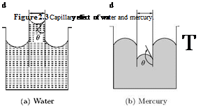
An associated effect of surface tension is the capillary deflection of liquids in small tubes. Examine the level of water and mercury in capillaries, shown in Figure 2.3.

When a glass tube is inserted into a beaker of water, the water will rise in the tube and display a concave meniscus, as shown in Figure 2.3(a). The deviation of water level h in the tube from that in the beaker

can be shown to be:

о

h a cos 9, (2.13)

d

where 9 is the angle between the tangent to the water surface and the glass surface. In other words, a liquid such as water or alcohol, which wets the glass surface makes an acute angle with the solid, and the level of free surface inside the tube will be higher than that outside. This is termed capillary action. However, when wetting does not occur, as in the case of mercury in glass, the angle of contact is obtuse, and the level of free surface inside the tube is depressed, as shown in Figure 2.3(b).

Another important effect of surface tension is that a long cylinder of liquid, at rest or in motion, with a free surface is unstable and breaks up into parts, which then assume an approximately spherical shape. This is the mechanism of the breakup of liquid jets into droplets.

The ratio of specific heats:

is an important parameter in the study of high-speed flows. This is a measure of the relative internal complexity of the molecules of the gas. It has been determined from kinetic theory of gases that the ratio of specific heats can be related to the number of degrees of freedom, n, of the gas molecules by the relation:

At normal temperatures, there are six degrees of freedom, namely three translational and three rotational, for diatomic gas molecules. For nitrogen, which is a diatomic gas, n = 5 since one of the rotational
degrees of freedom is negligibly small in comparison with the other two. Therefore:

Y = 7/5 = 1.4.

Monatomic gases, such as helium, have 3 translational degrees of freedom only, and therefore:

Y = 5/3 = 1.67.

This value of 1.67 is the upper limit of the values which the ratio of specific heats y can take. In general Y varies from 1 to 1.67, that is:

The specific heats of a gas are related to the gas constant R. For a perfect gas this relation is:

We know from thermodynamics that heat is energy in transition. Therefore, heat has the same dimensions as energy and is measured in units of joule (J).

2.2.5 Specific Heat

The inherent thermal properties of a flowing gas become important when the Mach number is greater than 0.5. This is because Mach 0.5 corresponds to a speed of 650 km/h for air at sea level state, therefore

for flow above Mach 0.5, the temperature change associated with velocity becomes considerable. Hence, the energy equation needs to be considered in the study and owing to this both thermal and calorical properties need to be accounted for in the analysis. The specific heat is one such quantity. The specific heat is defined as the amount of heat required to raise the temperature of a unit mass of a medium by one degree. The value of the specific heat depends on the type of process involved in raising the temperature of the unit mass. Usually constant volume process and constant pressure process are used for evaluating specific heat. The specific heats at constant volume and constant pressure processes, respectively, are designated by cv and cp. The definitions of these quantities are the following:

where u is internal energy per unit mass of the fluid, which is a measure of the potential and more particularly the kinetic energy of the molecules comprising the gas. The specific heat cv is a measure of the energy-carrying capacity of the gas molecules. For dry air at normal temperature, cv =717.5 J/(kg K). The specific heat at constant pressure is defined as:

where h = u + pv, the sum of internal energy and flow energy is known as the enthalpy or total heat constant per unit mass of fluid. The specific heat at constant pressure cp is a measure of the ability of the gas to do external work in addition to possessing internal energy. Therefore, cp is always greater than cv. For dry air at normal temperature, cp = 1004.5 J/(kg K).

Note: It is essential to understand what is meant by normal temperature. For gases, up to certain temper­ature, the specific heats will be constant and independent of temperature. Up to this temperature the gas is termed perfect, implying that cp, cv and their ratio у are constants, and independent of temperature. But for temperatures above this limiting value, cp, cv will become functions of T, and the gas will cease to be perfect. For instance, air will behave as perfect gas up to 500 K. The temperature below this liming level is referred to as normal temperature.

The change in volume of a fluid associated with change in pressure is called compressibility. When a fluid is subjected to pressure it gets compressed and its volume changes. The bulk modulus of elasticity is a measure of how easily the fluid may be compressed, and is defined as the ratio of pressure change to volumetric strain associated with it. The bulk modulus of elasticity, K, is given by:

Pressure increment dp

K = ———————– = -V—

Volume strain dV

It may also be expressed as:

where v is specific volume. Since dp/p represents the relative change in density brought about by the pressure change dp, it is apparent that the bulk modulus of elasticity is the inverse of the compressibility of the substance at a given temperature. For instance, K for water and air are approximately 2 GN/m2 and 100 kN/m2, respectively. This implies that air is about 20,000 times more compressible than water. It can be shown that, K = a2/p, where a is the speed of sound. The compressibility plays a dominant role at high-speeds. Mach number M (defined as the ratio of local flow velocity to local speed of sound) is a convenient nondimensional parameter used in the study of compressible flows. Based on M the flow is divided into the following regimes. When M < 1 the flow is called subsonic, when M & 1 the flow is termed transonic Bow, M from 1.2 to 5 is called supersonic regime, and M > 5 is referred to as hypersonic regime. When flow Mach number is less than 0.3, the compressibility effects are negligibly small, and hence the flow is called incompressible. For incompressible flows, density change associated with velocity is neglected and the density is treated as invariant.

The kinematic viscosity coefficient is a convenient form of expressing the viscosity of a fluid. It is formed by combining the density p and the absolute coefficient of viscosity m, according to the equation:

(2.5)

The kinematic viscosity coefficient v is expressed as m2/s, and 1 cm2/s is known as stoke.

The kinematic viscosity coefficient is a measure of the relative magnitudes of viscosity and inertia of the fluid. Both dynamic viscosity coefficient m and kinematic viscosity coefficient v are functions of temperature. For liquids, m decreases with increase of temperature, whereas for gases m increases with increase of temperature. This is one of the fundamental differences between the behavior of gases and liquids. The viscosity is practically unaffected by the pressure.

2.2.4 Thermal Conductivity of Air

At high-speeds, heat transfer from vehicles becomes significant. For example, re-entry vehicles encounter an extreme situation where ablative shields are necessary to ensure protection of the vehicle during its
passage through the atmosphere. The heat transfer from a vehicle depends on the thermal conductivity к of air. Therefore, a method to evaluate к is also essential. For this case, a relation similar to Sutherland’s law for viscosity is found to be useful, and it is:

( T3/z

к = 1.99 x 10 3 ( ———— I J/(s m K),

T + 112y

where T is temperature in kelvin. The pressure and temperature ranges in which this equation is applicable are 0.01 to 100 atm and 0 to 2000 K, respectively. For the same reason given for viscosity relation, the thermal conductivity also depends only on temperature.

The property which characterizes the resistance that a fluid offers to applied shear force is termed viscosity. This resistance, unlike for solids, does not depend upon the deformation itself but on the rate of deformation. Viscosity is often regarded as the stickiness of a fluid and its tendency is to resist sliding between layers. There is very little resistance to the movement of the knife-blade edge-on through air, but to produce the same motion through a thick oil needs much more effort. This is because the viscosity of the oil is higher compared to that of air.

2.2.3 Absolute Coefficient of Viscosity

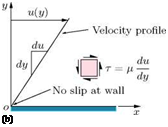
The absolute coefficient of viscosity is a direct measure of the viscosity of a fluid. Consider the two parallel plates placed at a distance h apart, as shown in Figure 2.2(a).

The space between them is filled with a fluid. The bottom plate is fixed and the other is moved in its own plane at a speed u. The fluid in contact with the lower plate will be at rest, while that in contact with the upper plate will be moving with speed u, because of no-slip condition. In the absence of any other influence, the speed of the fluid between the plates will vary linearly, as shown in Figure 2.2(b). As a direct result of viscosity, a force F has to be applied to each plate to maintain the motion, since the fluid will tend to retard the motion of the moving plate and will tend to drag the fixed plate in the direction of the moving plate. If the area of each plate in contact with fluid is A, then the shear stress acting on each plate is F/A. The rate of sliding of the upper plate over the lower is u/h.

These quantities are connected by Maxwell’s equation, which serves to define the absolute coefficient of viscosity p. Maxwell’s definition of viscosity states that:

“the coefficient of viscosity is the tangential force per unit area on either of two parallel plates at unit distance apart, one fixed and the other moving with unit velocity”.

T

(a)

Figure 2.2 Fluid shear between a stationary and a moving parallel plates.

Maxwell’s equation for viscosity is:

F u

A = gU

Hence,

[ML-1 T-2] = [g] [LT-1L-1] = [g] [T-1]

that is,

[g] = [ML-1T-1] .

Therefore, the unit of g is kg/(m s). At 0 °C the absolute coefficient of viscosity of dry air is 1.716 x 10-5 kg/(ms). The absolute coefficient of viscosity g is also called the dynamic viscosity coefficient.

The Equation (2.2), with g as constant, does not apply to all fluids. For a class of fluids, which includes blood, some oils, some paints and so called “thixotropic fluids,” g is not constant but is a function of du/dh. The derivative du/dh is a measure of the rate at which the fluid is shearing. Usually g is expressed as (N. s)/m2 or gm/(cm s). One gm/(cm s) is known as a poise.

Newton’s law of viscosity states that “ the stresses which oppose the shearing of a fluid are proportional to the rate of shear strain,” that is, the shear stress т is given by:

where g is the absolute coefficient of viscosity and du/dy is the velocity gradient. The viscosity g is a property of the fluid. Fluids which obey the above law of viscosity are termed Newtonian fluids. Some fluids such as silicone oil, viscoelastic fluids, sugar syrup, tar, etc. do not obey the viscosity law given by Equation (2.3) and they are called non-Newtonian fluids.

We know that, for incompressible flows, it is possible to separate the calculation of velocity boundary layer from that of thermal boundary layer. But for compressible flows it is not possible, since the velocity and thermal boundary layers interact intimately and hence, they must be considered simultaneously. This is because, for high-speed flows (compressible flows) heating due to friction as well as temperature changes due to compressibility must be taken into account. Further, it is essential to include the effects of viscosity variation with temperature. Usually large variations of temperature are encountered in high-speed flows.

The relation m(T) must be found by experiment. The voluminous data available in literature leads to the conclusion that the fundamental relationship is a complex one, and that no single correlation function can be found to apply to all gases. Alternatively, the dependence of viscosity on temperature can be calculated with the aid of the method of statistical mechanics, but as of yet no completely satisfactory theory has been evolved. Also, these calculations lead to complex expressions for the function /г(Т). Therefore, only semi-empirical relations appear to be the means to calculate the viscosity associated with compressible boundary layers. It is important to realize that, even though semi-empirical relations are not extremely precise, they are reasonably simple relations giving results of acceptable accuracy. For air, it is possible to use an interpolation formula based on D. M. Sutherland’s theory of viscosity and express the viscosity coefficient, at temperature T, as:

M = ( T_3/2 To + S Mo To) T + S

where mo denotes the viscosity at the reference temperature T0, and S is a constant, which assumes the value 110 K for air.

For air the Sutherland’s relation can also be expressed [1] as:

where T is in kelvin. This equation is valid for the static pressure range of 0.01 to 100 atm, which is commonly encountered in atmospheric flight. The temperature range in which this equation is valid is from 0 to 3000 K. The absolute viscosity is a function of temperature only because, in the above pressure and temperature ranges, the air behaves as a perfect gas, in the sense that intermolecular forces are negligible, and that viscosity itself is a momentum transport phenomenon caused by the random molecular motion associated with thermal energy or temperature.

In any form of matter the molecules are continuously moving relative to each other. In gases the molecular motion is a random movement of appreciable amplitude ranging from about 76 x 10-9 m, under normal conditions (that is, at standard sea level pressure and temperature), to some tens of millimeters, at very low pressures. The distance of free movement of a molecule of a gas is the distance it can travel before colliding with another molecule or the walls of the container. The mean value of this distance for all molecules in a gas is called the molecular mean free path length. By virtue of this motion the molecules possess kinetic energy, and this energy is sensed as temperature of the solid, liquid or gas. In the case of a gas in motion, it is called the static temperature. Temperature has units kelvin (K) or degrees celsius (°C), in SI units. For all calculations in this book, temperatures will be expressed in kelvin, that is, from absolute zero. At standard sea level condition, the atmospheric temperature is 288.15 K.

2.2.2 Density

The total number of molecules in a unit volume is a measure of the density p of a substance. It is expressed as mass per unit volume, say kg/m3. Mass is defined as weight divided by acceleration due to gravity. At
standard atmospheric temperature and pressure (288.15 K and 101325 Pa, respectively), the density of dry air is 1.225 kg/m3.

Density of a material is a measure of the amount of material contained in a given volume. In a fluid system, the density may vary from point to point. Consider the fluid contained within a small spherical region of volume SV, centered at some point in the fluid, and let the mass of fluid within this spherical region be Sm. Then the density of the fluid at the point on which the sphere is centered can be defined by:

There are practical difficulties in applying the above definition of density to real fluids composed of discrete molecules, since under the limiting condition the sphere may or may not contain any molecule. If it contains, say, just a single molecule, the value obtained for the density will be fictitiously high. If it does not contain any molecule the resultant value of density will be zero. This difficulty can be avoided over the range oftemperatures and pressures normally encountered in practice, in the following two ways:

1. The molecular nature of a gas may be ignored, and the gas is treated as a continuous medium or continuous expanse of matter, termed continuum (that is, does not consist of discrete particles).

2. The decrease in size of the imaginary sphere may be assumed to reach a limiting size, such that, although it is small compared to the dimensions of any physical object present in a flow field, for example an aircraft, it is large enough compared to the fluid molecules and, therefore, contains a reasonably large number of molecules.