COMPUTATION OF THE STANDARD INTERCONNECTION STRUCTURE
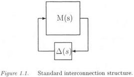
Consider an LTI closed loop subject to parametric uncertainties and neglected dynamics. Simple examples illustrate in the following subsections that it is most generally possible to transform a specific uncertain closed loop into the standard interconnection structure M(s) – A(s) of Figure 1.1: the transfer matrix M(s) contains the dynamics of the nominal closed loop (i. e. the closed loop without any model uncertainty) and the way the various model perturbations enter the closed loop. On the other hand, all model perturbations are gathered in the uncertain transfer matrix A(S). As a preliminary, the notion of LFT, which plays a key role in the Ц framework (and more generally in robust control and robustness analysis), is defined.
|
|
1.1 LFTS
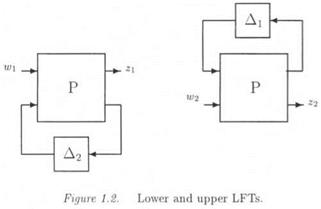
Lower and upper LFTs are defined in this subsection in a generic way. Let P, Ді, Д2 denote either transfer matrices or complex matrices: in Figure 1.2, the lower LFT F)(P, Д2) is the transfer between w and z, while the upper LFT FU(P, Ai) is the transfer between u;2 and г2. Partitioning P compatibly with the Aj’sas:
|
|
the LFTs Fi{P, Д2) and FU{P, Ai) can be written as:
Fl(P, Д2) = Pn + P2&2(I – P22&2)~XP2
Fu(P, Al) = P22+P2lbl(I-Pnbl)~lPl2 (1.2)
|
|


