Category FLIGHT MECHANICS MODELING and ANALYSIS

The uncertainty bounds for parameter estimates obtained from the Cramer-Rao bounds/OEM are multiplied with a fudge factor to reflect the uncertainty correctly. This is because when the OEM (which does not handle the process noise) is used on flight data, which are often affected by the process noise (like atmospheric turbulence), the uncertainty bounds do not correctly reflect the effect of this noise on the uncertainty of the estimates. And hence a fudge factor of about 3 to 5 can be used in practice.

TABLE C2 Design Approaches and Performance Specifications
Bode Plots/Frequency Responses	Nichols Charts/Frequency Responses
Time-Domain/Optimala Pole Placement Method Control Methods
Root Locus
Performance criteria to be specified	Coefficients of steady-state errors/phase margins/crossover frequency	Coefficients of steady-state errors/maximum closed loop frequency response and frequency	Coefficients of steady-state errors/location of dominant poles of the closed loop and root sensitivity Cascade lead, lag, feedback	Desired closed loop TF, poles sensitivities to parameter variations More general ones in feed forward, feedback, or both	Integral performance criteria in time domain
Compensation Cascade lead, lag, or types lead-lag	Cascade lead, lag, or lead-lag
Varieties of optimization methods are used for obtaining the optimum input to the plant
Source: Sinha, N. K. Control Systems. Holt, Rinehart and Winston, Inc. 1988. a There is a huge body of literature on optimal/modern control methods. Besides these, the approaches based on quantitative feedback theory, H-infinity, and hybrid (H2/H-infinity) methods are also used.

This number has been arrived at (on the average) by performing flight simulations – based parameter-estimation exercises for a fighter aircraft for longitudinal and

lateral-directional maneuvers and using the formula FF = Jn sa™plinf frequenC^—.

° V (2 bandwidth of residuals)

C10 GENETIC ALGORITHMS

Genetic algorithms are heuristic/directed search methods and computational models of adaptation and evolution based on the natural selection strategy of evolution of biological species. The search for beneficial adaptations to a continually changing environment in nature (i. e., evolution) is fostered by the cumulative evolutionary knowledge that each species possesses of its forebears. This knowledge, which is encoded in the chromosomes of each member of a species, is passed from one generation to the next by a well-known mating process wherein the chromosomes of ‘‘parents’’ produce ‘‘offspring.’’ Thus, genetic algorithms mimic and exploit the genetic dynamics underlying natural evolution to search for optimal and global solutions of general combinatorial optimization problems. The applications are the traveling salesman problem, VLSI circuit layout, gas pipeline control, the parametric design of an aircraft, learning in neural nets, models of international security, strategy formulation, and parameter estimation.

[1] dL

Ix dp

[3] Using a 4DOF lateral-directional model, find the eigenvalues for spiral, roll, and DR mode, and (3) determine the roots using DR approximation. Compare the results with those obtained in (2) and comment.

5.6 How would you get the flight path rate from acceleration and subsequently the body rate?

5.7 Will large or small changes occur in the airspeed in the SP transient mode?

5.8 What is the main distinction between SP and phugoid mode characteristic from the motion of the aircraft and the interplay of the forces and moments?

A control system might need some adjustments in order that several conflicting requirements can be adequately met. These adjustments are called compensations.

A compensator can be inserted either in the forward or feedback paths, or in both the paths. In hardware control systems, the compensators are some physical devices that are electrical, mechanical, or hydraulic/pneumatic. In digital control systems, wherein the control laws are computer programs, the compensators are also com­puter programs and work equivalently to the HW devices. A lead compensator can be used to provide a phase lead between the output and the input. Similarly lag and lead-lag compensators are used as the case may be. The main idea is to modify the frequency response of the open loop system/TF such that the performance of the compensated closed loop system is satisfactory. Table C2 gives an overview of various approaches used for control system design.

Root Locus

The method is based on the fact that it is possible to adjust the location of the poles of the closed loop TF by varying the loop gain. The root locus sketches the movement in the s-plane of the poles of the closed loop TF as open loop gain or some parameter is varied from zero to infinity. Let the characteristic polynomial of the closed loop system be represented as KP(s) + Q(s) = 0, with K as some parameter to be varied from zero to infinity to obtain the plots of the roots of this equation leading to the root locus. It can be represented in the form: 1 + KP(s)/Q(s) = 0 or Kq(| = — 1 = 1ff180°. This will yield the basic conditions to be satisfied by all the points on the root locus: (1) the angle condition—at a point on the root locus the algebraic sum of the angles of vectors drawn to it from the open loop poles and zeros is an odd multiple of 180° and (2) the magnitude condition—at a point on the root locus the value of K is given as

product of lengths of the vectors from poles

K =

product of lengths of the vectors from zeros

The angle condition tells us if any point in the s-plane lies on the root locus, and the magnitude condition gives the value of K for which this point will be a root of the characteristic equation. Important properties of the root locus are as follows: (1) it is symmetrical about the real-axis of the s-plane, (2) a root locus branch starts from each open loop pole and terminates at each open loop zero or infinity, (3) the number of branches that terminate at infinity is equal to the number of open loop poles less the number of open loop poles, (4) the sections of the real axis to the left of an odd number of poles and zeros are part of the locus, for K > 0, and (5) if the number of poles and zeros are odd and to the right of a point, then this point is on the root locus.

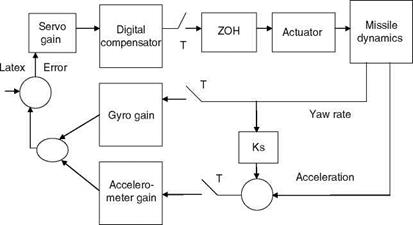
Digital computers are increasingly being used to implement control systems and for many related studies. Most modern control systems operate in the digital domain. Control system laws are computed via algorithms in a digital computer. One can view the computer-controlled systems as an approximation of analog-control systems.

In such a system the signal conversion is done at tk, the sampling instant (or time) (Figure C3). The system runs open loop in the interval between the A-D and the D-A conversion (analog to digital and digital to analog), and the computational events in the system are synchronized by the real-time clock in the computer. Such a system is a sampled-data system, but the events are controlled and monitored by a computer or its dedicated microprocessor (chip). The D-A converter produces a continuous-time signal by keeping the control signal constant between the signal conversions. These signals are called sampled or discrete-time signals. Thus, we can use the term sampled data system synonymously for the computer-controlled system. In terms of the system – theoretic concept a computer-controlled system with periodic sampling is a periodic system because if a system is controlled by a clock, the response of the system to an external stimulus will then depend on how the external event is synchronized with the internal clock of the computer system. A digital control system would have several merits: (1) there is freedom from direct bias and drift of the analog computers, (2) desired accuracy can be obtained by proper implementation of the control algorithms in the computer, (3) generally there is no data storage limitation, (4) time-sharing ability of the digital computer can be used to advantage for reducing the cost of implementation/computation, (5) effect of quantization and sampling can be mod­eled and studied in advance of the implementation of the control strategies, (6) adaptive and reconfiguration control algorithms can be implemented with ease, and

(7) fuzzy logic-based control systems can be easily implemented.

Before any postflight data analysis for parameter estimation and related work is carried out, it would be desirable to preprocess the data to remove spurious spikes

and any high-frequency noise: (1) edit the data to remove wild points and replace the missing points (often an average from two samples is used), (2) filter the edited/raw data to reduce the effect of noise, and (3) decimate the data to obtain the data at the required sampling rate for further postprocessing; for this the data should have been filtered at a higher rate than required. Editing by using the finite – difference method and filtering using FFT (fast Fourier transform)/spectral analy­sis can be done. The editing is a process of removing the data spikes (wild points) and replacing them with suitable data points. Wild points occurring singly can be detected using the slope of the data set or first finite difference. Any data point exhibiting higher than the prefixed slope is considered as a wild point and eliminated. When wild points occur in groups, the surrounding points are con­sidered to detect them. A finite-difference array consisting of first-, second-, and third-difference (up to nth differences) is formed. The maximum allowable upper and lower limits for these differences are pre-specified and if the array indicates any value greater than the limits, the points are treated as wild points and eliminated. The points are replaced by suitable points by interpolation, considering surrounding points. If the editing limits are too high, the edited data will leave a large amount of wild points, and if the limit is too small, the edited data would appear distorted.

Filtering is the process of removing the noise components presented in the edited/raw data. These filters introduce the time lag effects in the flight data, thereby compounding the problem of parameter estimation. Discrete Fourier transform (DFT) method allows processing from time domain to frequency domain and does not introduce time lags. However, it is an offline procedure. Based on spectral analysis through DFT, one can know the frequency contained in the raw signal. Nowadays, filtering/editing can be easily carried out using certain functions from the MATLAB signal processing tool box. However, certain fundamental aspects are described briefly here.

The Fourier transform (FT) from time to frequency domain is given by

Here, h(t) is the time function of the signal, H(t) is the complex function in frequency domain, and N is the number of samples.

The inverse FT (from frequency to time domain) is given by

h(t)	(C4)

Here, H*(f) is the conjugate of H(f), and * is for the conjugate operation. By comparing Equations C2 and C4, it can be seen that the same transformation routine can be used. After the inverse transformation, the conjugate is not necessary because the data in time domain are real. The signal to be filtered is first transformed into frequency domain using DFT. Using cutoff frequency, the Fourier coefficients of the unwanted frequencies are set to zero. Inverse FT time domain yields the filtered signal. For proper use of the filtering method, selection of the cutoff frequency is crucial. In spectral analysis method, the power spectral density of the signal is plotted against frequency and the inspection of the plot helps distinguish the frequency contents of the signal. This information is used in selecting the proper cutoff frequency for the filter. The FT of the correlation functions are often used in analysis. The FT of the autocorrelation function (ACF) 1

fxx(T) exp(—jvT) dT

— 1

is called the power spectral density function of the random process x(t). The ‘‘power’’ term here is used in a generalized sense and indicates the expected squared value of the members of the ensemble. fxx(v) is indeed the spectral distribution of power density for x(t) in that integration of fxx(v) over frequencies in the band from v1 to v2 yields the mean-squared value of the process, whose ACF consists only of those harmonic components of fxx(T) that lie between these frequencies. The mean – squared value of x(t) is given by the integration of the power density spectrum for the random process over the full range of frequencies:

—1

This is an important ingredient of the total flight testing, simulation, and estimation exercises. For successful data analysis a good set of data should be generated, gathered, and recorded or telemetered. The data acquisition personnel and data analysts should keep several aspects in mind: (1) How the data got to the analysis program from the sensors and how the data were filtered, (2) How the data were digitized, time tagged, and recorded, and (3) For extracting more information from data as much information as available from the related sources should be recor – ded/gathered. This requires a systems approach. This is to say that one should look at the entire system from input to output because the connections and interactions between various components are of varied nature and importance. One should safeguard against over reliance on misleading simulation, unforeseen circumstances, and neglect of the synergism of data system problems.

In most of the flight mechanics modeling and analysis exercises, digitized data are required. It is important to see that the sampling rate is properly selected so that there is no loss of useful information and that the burden of collecting too much data does not increase. It is based on the Nyquist theory, which applies to many different fields where data are captured. In general terms, it states the minimum number of resolution elements required to properly describe or sample a signal. In order to reconstruct (interpolate) a signal from a sequence of samples, sufficient samples must be recorded to capture the peaks and trough of the original waveform. For example, when a digital recording uses a sampling rate of 50 kHz, the Nyquist frequency is 25 kHz. If a signal that is sampled contains frequency components that are above the Nyquist limit, aliasing will be introduced in the digital representation of the signal unless those frequencies are filtered out before digital encoding. The Nyquist sampling theorem states that a sample with a regular sample interval of T seconds (a sample rate of 1/T samples/s) can contain no information at a frequency higher than 1/(2T) Hz. This limit frequency is called the Nyquist frequency, the half-sample frequency, or the folding frequency. Frequency limits of 12.5 or 25 Hz (25 or 50 samples/s) are sufficient to include all useful aircraft stability and control informa­tion on the modes/data. The higher frequencies in the original continuous-time signal could contain (1) structural resonance modes, higher than the rigid body dynamic modes, (2) AC (altering current) power frequencies, (3) engine vibration modal responses, and (4) thermal noise and other nuisance data. These high-frequency data shift to an apparent lower frequency and this phenomenon is called aliasing or frequency folding (Nyquist folding). The high-frequency noise/data contaminate the low-frequency stability and control data. After sampling there is no way to remove

Low frequency—affected FIGURE C2 Frequency aliasing.

the effect of this aliasing, and hence the data should be adequately treated before sampling. The effective method is to apply pre-sample filtering to the data. This means filtering the signal (+noise, or unwanted higher frequency data) to remove the high-frequency/unwanted data/responses before the actual sampling is performed. To avoid the aliasing effect, (1) pre-filter the data before digitization, so that unwanted signals in the higher band that would otherwise aliase the low frequencies would be eliminated; however, the pre-filtering would introduce lags in signal, so the time lag should be accounted for and (2) sample the signal at a very high rate, so that the folding frequency is moved farther away and the high-frequency signals (noise, etc.) would alias the frequencies that are near the new folding frequency, which is farther away from the system/signal frequency of interest. This assures that the useful low-frequency band signals are not affected, as can be seen from Figure C2.

However, it is prudent to sample the aircraft responses at 100 or 200 samples/s and then digitally filter the data and thin it to 25 or 50 samples/s. The pre-sample filter requirements are (1) a low-pass filter at 40% of the Nyquist frequency can be used, (2) for systems with high sampling rates, a first-order filter would be adequate, and (3) for low sample rate systems higher-order filters may be necessary.

In the digitized signal, the resolution is exactly one count, and if the resolution magnitude is much smaller than the noise level of the digitized signal, the resolution problem is a non-issue. A good resolution is 1/100 of the maneuver size and a low resolution is acceptable for Euler angles, say, 1/10 of the maneuver size. The time tagging of data is very important. The time errors, in data measurements, would affect the accuracy of estimated derivatives depending on the severity of these errors. ‘‘Time tagging’’ refers to the information about the time of each measurement. Any time lag due to analog pre-filtering or sensors should be taken into account; otherwise, it would cause errors in time tag. Some derivate estimates are extremely sensitive to time shifts in certain signals. Time errors >0.01 s may cause problems, whereas accuracy of 0.02-0.05 s is usually tolerable for signals like altitude and airspeed.

CRITERION, NYQUIST CRITERION, GAIN/PHASE MARGINS

A linear spring-mass system is described as (Figure 2.5)

Mx + Dx + Kx = 0 (C1)

Assume that mass M is displaced to the right by a small disturbance x. When the displacement takes place, the spring with its stiffness K (if K is positive) will provide a restoring force proportional to Kx to the mass. The positive restoring force is because K is positive and it is in the direction opposite to the initial movement of the object. The mass will have an initial tendency to move toward the original position. This is the static stability of a dynamic system. If K is negative then naturally the mass will keep moving in the forward direction, since the spring force will be in the direction of x. The mass will further move away from the original equilibrium

TABLE C1

Steady-State Error for Types of Systems

position. This condition is called static instability. The differential Equation C1 has two roots:

Routh-Hurwitz Criterion

The characteristic equation of the control system is its denominator equated to zero. The Routh-Hurwitz (RH) criterion relates to studying the characteristic equation: (1) the control system is dynamically stable if all the roots have negative real parts, (2) the system is unstable if any root has a positive real part, and (3) the system is neutrally or marginally (stable/unstable) if one or more roots have pure imaginary values. Let this equation be given as g(s) = ansn + an-1sn-1 + ••• + a1s + a0. Now, construct the Routh array as shown. The first two rows are obtained from the characteristic equation. The remaining element of the Routh array are calculated from the following expressions: bn-1

1-. an-1an-4 anan-5 • ~ .

bn-3 =———————— ~1—————– ; —Cn—1~———— b„-1

the sign changes in the elements of the first column of the array. This number signifies the number of roots with positive real parts. If there are no sign changes, then the system is stable.

Nyquist Criterion

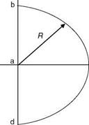
We can examine the frequency response of the G(s)H(s) (or GH(s)) loop TF and see if the gain is greater than unity at the phase lag of 180°. This is equivalent to studying the condition GH( jv) = -1 or finding a root of (GH + 1) on the s-plane jv axis, this being the stability boundary. The stability of the system is studied by using the principle of an argument advanced by Nyquist. A semicircular contour of infinite radius is used to enclose the right hand s-plane (RHS). According to this principle, as s traverses the closed contour in a clockwise direction, the increment in the argument

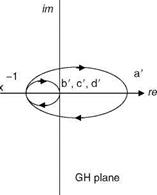FIGURE C1 Nyquist contour (R is infinite radius) and Nyquist plot.

of (1 + GH) is 2pN. Now, if P = the number of the poles of GH + 1 and Z = the number of zeros of GH + 1 inside the Nyquist contour (i. e., the right hand s-plane with infinite radius), then N = P — Z, the number of counterclockwise encirclements of the origin of the s-plane. This can be translated to count the encirclements of the critical point — 1 + j0 by the GH. The stability criterion is specified as Z = P — N. We recognize here that the poles of 1 + GH are the open loop poles and the zeros of 1 + GH are the closed loop poles. Thus, the number of the unstable closed loop poles is equal to the number of the unstable open loop minus the number of the counter­clockwise encirclements of the critical point. The steps involved in the determination of the stability of the system using the Nyquist plot are illustrated in Figure C1 for the following TF [1]:

(s + 1)(s + 2)(s + 5)’

(1) The part ab of the Nyquist contour is the jv axis from v = 0 to v = 1. This maps to the Nyquist polar from a’ to b’ (the latter at the origin), (2) The infinite semicircle bcd maps into the origin of the polar plot of GH = plane, i. e., into points b’, c’, and d’, and (3) The negative jv axis da maps into the curve d’a’ in the GH-plane. We see that the GH-plane Nyquist plot does not enclose the critical point, and hence N = 0. Since P = 0 (there are no poles of the GH in the RHS plane) hence Z = 0, meaning that there are no closed loop poles in the RHS plane. The closed loop system is stable.

Gain/Phase Margins

We see from the RH criterion that it gives the absolute stability of the system, i. e., whether the system is stable or unstable. The gain/phase margins give the relative stability of the system. They measure the nearness of the open loop frequency response to the critical point. The gain margin (the GH frequency response is plotted)
from the point where the phase lag is 180°, is the additional gain needed to make the system just unstable, whereas the phase margin (from the point where the gain is one) is the additional phase lag needed to render the system just unstable. The margins for a given system can be easily computed using the MATLAB control system toolbox. Gain and phase margins are the criteria specified for the design of control systems. What is almost always specified is that the gain margin (of the loop TF GH(s)) should be at least 6 dB, and the phase margin should be at least 45°.

Any dynamic control system can be subjected to analysis to see if it meets certain performance criteria. The performance of the control system is studied in terms of its transient – and steady-state behavior. The first is the response to the initial conditions and the latter the response when the transients are settled. Since these two require­ments are often conflicting, a trade-off is required. The responses of a system are studied in terms of unit step-, unit ramp-, and unit-parabolic inputs. As seen in Chapters 7 and 9, the responses of a dynamic system can be obtained by applying short pulse, doublet, 3-2-1-1, and other multi-step inputs for studying the specific behavior of such systems. Often a steady-state error in standard inputs to a control system is computed. The highest power of s in the denominator of the TF is equal to the order of the highest derivative of the output, and if this highest power is equal to n, the system is an order ‘‘n.’’ A system could have a pole at origin of multiplicity N. Then it is of type N. This signifies the number of integrations involved in the open loop system. If N = 1, then the system is of type 1, if N = 0, then it is type zero, and so on. The steady-state error in terms of the gain K of the system is given in Table C1. If the type number of the system is increased, the accuracy for the same type of input is increased, but the stability of the system is aggravated progressively.

A dynamic system could be stable or unstable. Even if such a system is stable, its performance might not be satisfactory. Therefore, in general one can say that all such systems would need some regulation, regulatory mechanism, or control of the variables to improve and enhance the performance of the system. A system that functions under partial of full supervision or control of some ‘‘control mechanism’’ (which could be regulatory control, feedback control, or feed forward control) is in every sense called a control system. In general control system analysis, say for an airplane, can be carried out using frequency-domain or time-domain methods. Frequency-domain methods are based on Bode diagrams, root locus, Nichols charts, and transfer functions. Direct time-domain analysis can be done using state-space methods. Due to easy availability of high-speed computers, any time-consuming technique can be easily adapted for analysis, design, and evaluation of control systems. The MATLAB/SIMULINK SW tool and its tool kit are convenient ways for such analysis. These tools can be easily learned and practiced and can save a lot of time and effort in carrying out detailed analysis and validation of control system designs.

The transfer function (Equation 2.1) for linear systems is defined in terms of Laplace transforms (LT). For a function/(f), the LT is defined as L(s) = J0° f (t)e~st df. For example, the LT of unit step input u is given as 1/s; s is the complex frequency s = s + jv. We can see that the function f(t) need not be periodic. The inverse LT is defined as f (t) = щ 1^°° L(s)est ds. If s in the TF is replaced by jv, we obtain the complex numbers with respect to frequency. If the input is a sign wave, then we get the steady-state output as a sign wave of the same frequency, but with different magnitudes and phase angle differences between output and input waves. The plot of these complex numbers with respect to frequency is called the frequency response.

Bode diagram is a plot of magnitude (or amplitude ratio) and the phase angle (phase difference between the output and input) of a TF vs. frequency (Figure 2.4). In definition, the Bode plot is the result of the plot of magnitude and phase of poles and zeros of the TF with respect to frequency in logarithmic coordinates. The simplification in Bode plots is because in logarithmic representation, multiplication and division are replaced by addition and subtraction, respectively. In a filter or control system’s Bode diagram, the cutoff frequency is the point where the response is 3 dB down in amplitude from the level of the pass band. Beyond this frequency, the filter will attenuate (the amplitude) at all other frequencies.

Several concepts from linear control/systems theory are collected in nearly alpha­betical order [1-4]. All of which might have not been used in this book; however, they would be very useful in general for aerospace science and engineering applications.

C1 CONTROL SYSTEM: A "DYNAMICAL SYSTEM” CONCEPT

A system is something that can be studied as a whole. It is a collection of parts, subsystems, or components that function in unison to enable the system to carry out an assigned functional role. An airplane is a complex and sophisticated dynamic system in this sense. Systems may consist of subsystems that are interesting in their own right (Chapter 6). They may exist in an environment that consists of other similar systems. Systems are generally understood to have an internal state, inputs from an environment, and methods for manipulating the environment or themselves. Since cause and effect can flow in both directions of a system and environment, interesting systems often possess feedback. The idea behind dynamic systems theory is studying, understanding, and estimating the long-term behavior of a system that changes in time. The characterization of this behavior consists in knowing the conditions of a system. Some examples of these are (1) the system has a periodic behavior, (2) it recurrently returns to a given set, (3) it goes to all the possible sets that cover its space, (4) it never leaves a given set, and (5) its components interact with each other as desired.

Although there is a clear distinction between the so-called ‘‘classical’’ (frequency domain-based) and ‘‘modern’’ (time domain/optimal control) concepts and theories, we do not want/need to invoke these distinctions here. These are matters of the past and of a bygone era! Even today we need to use tools or techniques available easily for analysis and design of systems/control systems. The point is that with the great progress in computing technology (HW memory, speed, HW/SW parallelization) we can easily use any of the classical or modern tools with greater ease and flexibility than we could do two decades ago. And we believe that we need to use Bode diagrams and transfer functions to have the frequency domain feel and interpretation as well as state-space and time-domain analysis for optimization and direct time – history visualization and interpretation of control system performance. Hence, we should use both approaches in an integrated way to achieve the best design with the best performance. We should perhaps call this a hybrid approach rather than classical or modern. Also, since even this hybrid approach would further be augmented using ‘‘soft computing’’ (based on artificial neural networks, fuzzy logic/modeling, genetic algorithms, and approximate reasoning), we would like to consider the entire gamut of control system analysis, design, and validation methods as the ‘‘general theory of control systems.’’ The main reason for this is that we should make recourse to all or several such composite (classical, modern, and soft) approaches and tools for analysis, design, and validation of complex and sophisticated control systems: fly­by-wire aircraft, spacecraft, missiles, UVAs, MAVs, huge powerful computing network systems, and integrated electrical power grids/systems.

In a dynamic system simulation one can study the effect of random noise on parameter/state estimates to evaluate the performance of the estimator. We first get one set of estimated parameters; then we change the seed number for random number generator and add these random numbers to measurements as noise. We get esti­mates of the parameters with the new data. We can formulate a number of such data sets with different seeds and obtain parameters to establish the variability of the estimates across different realizations of the data. We next obtain the mean value and the variance of the parameter estimates using all the individual estimates from all these realizations. The mean of the estimates should converge to the true values. The approach can be used for any type of system. Depending on the problem’s complexity 500 simulation runs or as small as 20 runs could be used to generate average results.

B19 PROBABILITY AND RELATIVE FREQUENCY

Relative frequency is the value calculated by dividing the number of times an event occurs by the total number of times an experiment has been carried out. The probability of an event is then thought of as its limiting value when the experiment is carried out several times; the relative frequency of any particular event will settle down to this value. Probability is expressed on a scale from 0 to 1; a rare event has a probability close to 0 and a very common event has a probability of 1.

If X is a continuous random variable, there is a function p(x) (PDF) such that for every pair of numbers a < = b, P(a < = X < = b) = (area under p between a and b). The probability density function of a random variable with a standard normal/ Gaussian distribution is the normal curve. Only continuous random variables have probability density functions.

The probability distribution of a random variable specifies the chance that the variable takes a value in any subset of the real numbers, and the probability distribution of a random variable is completely characterized by the cumula­tive probability distribution function. The probability distribution of a discrete random variable can be characterized by the chance that the random variable takes each of its possible values. The probability distribution of a continuous random variable is characterized by its PDF. The Gaussian PDF is given by p(x) = exP (— ), with m as the mean and s2 as the variance of the

distribution. For the measured random variables, given the state x (or param­eters), the PDF is given by p(z|x) = (2p)„/2|R|1/2 exp(- 2 (z – Hx)TR-1(z – Hx)), with R as the covariance matrix of measurement noise.