Our heavyweight helicopter equal in the world does not have
In Rostov started production of the most load-lifting rotary-wing car The Russian holding «Helicopt[...]

Everything about aircrafts and helicopters. News and events in aviation worldwide. Civil, transportation, military helicopters and airplanes.

Everything about aircrafts and helicopters. News and events in aviation worldwide. Civil, transportation, military helicopters and airplanes.

Everything about aircrafts and helicopters. News and events in aviation worldwide. Civil, transportation, military helicopters and airplanes.

Everything about aircrafts and helicopters. News and events in aviation worldwide. Civil, transportation, military helicopters and airplanes.


The calculation procedure is now presented, in schematic form, and is the basis for a flow diagram. Each part of the calculation is presented as a complete entity, in programming terms a function procedure or subroutine, with the appropriate input and output data being specified. This gives a segmented structure to the overall method, which is recommended for implementation in a computer program. The main program forms the input/output of data leaving separate routines to perform the detailed calculations.
A.7.2 Atmospheric Parameters
This determines the air parameters used by the calculations to be determined directly from the altitude and ambient temperature. An ISA atmospheric model is used. The helicopter is assumed to remain within the troposphere. Normally this is the case but in some instances helicopters have achieved very high altitudes; however these are truly exceptional and do not invalidate the model proposed.
A.7.2.1 Input
• Altitude
• Sea-level air temperature (absolute temperature at sea level)
• Sea-level air density.
A.7.2.2 Output
• Density ratio (s)
• Absolute temperature ratio (У)
• Pressure ratio (d).
A.7.2.3 Calculation
The absolute temperature ratio is given by:
y AbTmpSea Level—Altitude x LapseRate
![]() AbTmpSea Level
AbTmpSea Level
1 Altitude x LapseRate
AbTmpSea Level
 |
||
The pressure ratio by:
The lapse rate of 6.5 °C per kilometre is used in the calculations.
[1] This was a collaborative programme, jointly sponsored by Westland Helicopters and the Ministry ofDefence, which embraced blade aerofoil section research between the Royal Aircraft Establishment (now Dstl) and Westland Helicopters. This research work developed the advanced rotor blade and tip design for the Westland Lynx helicopter. Its most public achievement was the world speed record of 249.1 mph by aircraft serial number XZ170, designation G-LYNX, on 11 August 1986 over the Somerset Levels.
[2] Helicopter control is based primarily on directing the thrust generated by the main rotor(s). It is normally accepted that this thrust force is in a direction perpendicular to the rotor disc – that is, the plane traced out by the blade tips. This plane can be altered in two ways. The first is to alter the direction of the rotor shaft taking the rotating blades with it. The second is to permit the blades to move in a direction normal to the rotation plane, known as flapping, which allows the rotor disc plane to change without requiring any direct change in the rotor shaft. The tilting of the thrust force will in due course cause the helicopter to change its flight attitude which will then take the rotor shaft with it.
[3] = 1 (2Л0)
The thrust force is also normalized in a manner very close to that used for fixed-wing lift – that is, the product of a pressure and an area. The pressure is the dynamic pressure seen at the
[4] Autorotation is an extremely important facility because in case of a power failure the rotor can continue to produce a thrust approximately equal to the aircraft’s weight, allowing a controlled descent to ground to be made. The term ‘ideal autorotation’ is used because in practice power is still needed to overcome the drag of the blades (profile power).
[5] Some of the figures here are revisions of figures in The Foundations of Helicopter Flight by Simon Newman, Elsevier, 1994.
[6] This is seen in extreme form with the Westland Lynx world speed record helicopter (G-LYNX), see Figure 7.7.
[7] Main rotor blade tip accelerations of 750-1000g are typical.
[8] The term ‘incidence’ requires a brief reflection. In fixed-wing terminology, it is often defined as the orientation of a data line in the wing/blade relative to the forward flight direction. Helicopter aerodynamics tends to use the term ‘pitch angle’ for this orientation and reserves incidence for the inclination of the data line to the local incident flow including any downwash velocity. This is consistent with the term ‘angle of attack’. For the present discussion, incidence is the angle of the fuselage to the airflow direction generated by the motion of the aircraft.
In order to examine the ability of a helicopter design to perform a given mission, the calculations described – where engine power and fuel consumption can be determined at any flight speed – can be assembled so the helicopter model can ‘fly’ a mission in a computer. The ease and immediacy of this procedure make it of direct use to a project assessment. There is one important consideration to be made. As the helicopter consumes fuel, the weight changes, which in turn affects the fuel consumption itself. So, in an ideal world, the calculation becomes circular. However, if the mission is ‘flown’ in small time steps, or mission legs, then an iterative scheme can be used to obtain an estimate of the fuel consumption rate over the leg/time period. The mission is then assembled by linking these individual mission legs where the value of the helicopter weight at the end of a particular leg becomes the start value for the succeeding leg. (Each leg will be defined by a fixed flight condition, particularly forward speed. However, if a climb or descent – at constant speed – is required the iterative scheme can still be used.) The mission may contain discrete weight changes of payload, such as changes in passenger/cargo payload or the deployment of ordnance. These can be incorporated by placing any such occurrence at the join of two mission legs and the weight change made in moving from one to its successor.
The iterative scheme to account for the changing helicopter weight is now described. For each leg the procedure begins with the calculation of the power and fuel consumption at the start weight of the leg. The duration of the leg can be obtained either by the time being explicitly stated or by dividing the range by the speed to give the time. This enables a first estimate of the weight change over the leg to be calculated. By subtracting half of that fuel usage from the start weight, a revised helicopter weight is thus obtained. Taking this new value of aircraft weight the calculation process is repeated and a new estimate for fuel usage is thus obtained. The two values of the fuel usage, over the leg, at the two weights are then compared. If they differ within a specified tolerance, the process is seen to have converged and the final estimate is adopted. If the fuel usage values do not lie within the tolerance, a revised mean aircraft weight is adopted
(by subtracting half of the latest fuel usage value from the start weight of the particular mission leg) and the process is repeated. This iteration continues until convergence to within the required tolerance is achieved.
To illustrate the method, the following calculations, based on a small utility helicopter, are presented.
The helicopter data used are given in Table A.4.
The fuel-flow variation with power, presented in (A.25), was obtained from public domain information (a leaflet obtained at an air show) and, using linear regression, the following
|
Table A.4 |
||
|
Parameter |
Symbol |
Value |
|
Rotor data: |
||
|
Number of blades |
Nm |
4 |
|
Nt |
4 |
|
|
Chord (m) |
Cm |
0.394 |
|
Ctl |
0.180 |
|
|
Radius (m) |
RM |
6.4 |
|
RT |
1.105 |
|
|
Tip speed (m/s) |
VTM |
218.69 |
|
Vtt |
218.69 |
|
|
Blockage |
Bm |
1.05 |
|
BT |
1.1 |
|
|
Induced-power factor |
kiM |
1.1 |
|
kiT |
1.2 |
|
|
Profile drag coefficient |
CD0M |
0.011 |
|
CD0T |
0.012 |
|
|
Fuselage data: |
||
|
Tail boom length (m) |
^BOOM |
7.66 |
|
D100 (N) |
D100 |
6226.9 |
|
Auxiliary power (kW) |
PAUX |
26.1 |
|
Transmission loss factor |
TRLF |
1.04 |
|
Engine data: |
||
|
Number of engines |
Ne |
2 |
|
Intercept |
ae |
46.5 |
|
Slope |
Be |
0.24 |
equation was obtained:
 |
|
Using the data detailed above, the variation of the main rotor power components with forward speed is shown in Figure A.3, namely induced, profile, parasite and total.
Forward Speed (m/s)
2^
![]()

![]()
![]()
![]()
![]()
![]()
![]()
 Ф
Ф
О
Q_
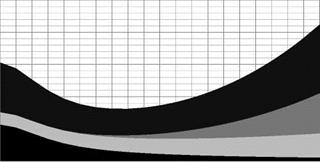
Figure A.4 Main rotor power components – cumulative
If these power components are viewed cumulatively, as in Figure A.4, the build-up of the total power can be seen.
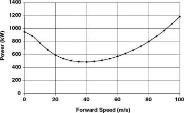
Having determined the total main rotor power, the total tail rotor power, the auxiliary power and the influence of the transmission losses, they can be combined to give the total overall power required of the engine(s).
This total power variation of the complete helicopter with forward speed is shown in Figure A.5.
 |
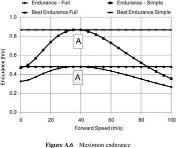
This power distribution now enables the fuel consumption to be calculated and by selecting a given weight of fuel to be consumed, the helicopter endurance and range can be calculated for the range of speeds. (For these calculations, the helicopter weight is considered constant.) Endurance, by definition, is the time required to consume that specified amount of fuel, and range is defined as the distance covered while consuming that fuel amount. It is apparent that endurance is focused on minimizing the rate of fuel usage with time, while range includes both time and speed and is therefore a compromise. (A fuel usage of 100 kg is assumed for these calculations.) The endurance is shown in Figure A.6, and the corresponding range (km) is
![]()
|
|
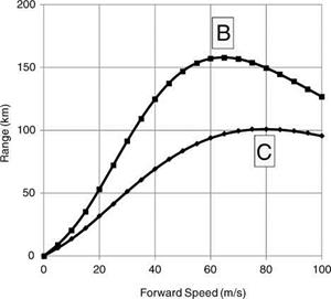
shown in Figure A.7. Each figure contains two plots referring to either the full fuel-flow law as defined in Equation A.26, or a modification to that law where the intercept (AE, or fuel flow at zero power) is set to zero. (Inspection shows that this corresponds to a constant sfc.) The lower curve corresponds to the full law (AE = 0) and the upper curve to the modified law (AE = 0) – where the fuel consumption rate (fuel flow) is smaller.
The positions of maximum endurance and range are indicated in the figures by a letter. Figure A.6 shows that the change in the fuel-flow law does not alter the best endurance speed of
|
Range – Full * Range – Simple
|
38 m/s (A), which, not surprisingly, corresponds to minimum power. However, because of the different fuel consumption rates, the change does have an influence on the best-range speed increasing it from 65 m/s (B) to 80 m/s (C) albeit with a smaller range.
Figure A.8 shows the best-range speeds, also indicated by B, and C, on the total power v forward speed curve.
In fact, the two points, B and C, corresponding to these ‘best’-range conditions, can be determined via a simple geometrical construction as the analysis below shows. Using the definitions in Table A.5, we have the following.
For point A (maximum endurance), the definition for sfc is:
![]() WFUEL
WFUEL
P • time
that is:
Endurance = WfUEL • — (A.28)
S P y ;
Since WFUEL and S are fixed values, the endurance is a maximum when P is minimum, that is point A is the minimum point on the power v velocity curve.

 |
Fuel weight (fixed) Power
Forward speed
Endurance
Range
For point B (maximum range – constant sfc, AE = 0), the range is given by:
Range = time • V
![]() _ V Wfuel
_ V Wfuel
= P • S
that is the range is a maximum (since WFUEL and S are fixed values) when P/V is a minimum, so point B is located where the tangent, drawn from the origin, touches the power curve.
For point C (maximum range – full fuel-flow law), in this we have:
Wfuel = time • (Ae + Be • P) (A.30)
Therefore:
Range = time • V
![]()
![]()
![]()
![]() (A.31)
(A.31)
This result is very similar to that defining point B except there is an additional term in the denominator (AE/BE). This means that the tangent has to be drawn from the point (0, — AE/BE). These constructions for the points B and C are shown in Figure A.8.
A.6.1 Influence of Wind
 |
||
If the helicopter is flying into a headwind of VW, the above formula for range becomes:
This means that the tangent should be drawn from the point (VW, —Ae/Be), as shown in Figure A.9.
 |
Figure A.9 Best-range speed with wind
So far, as regards the engine installation, the performance has been focused on the fuel consumption. During its operational life, a gas-turbine engine might be required to operate outside of normal continuous limits. In such circumstances, it will have limitations placed on it which are determined by the permissible operating temperature of the turbine section. So if the engine is required to operate at a power above the normal continuous limit, providing this occurs for a specified limited time period, it is possible to achieve this without causing
permanent damage. It may happen that a situation arises which can be considered to be an emergency and in order to save the helicopter, excessive wear or indeed damage to the engine(s) may be the only possible choice. These are also catered for, but the time limits are necessarily short. To illustrate this, typical examples of such power limitations are as follows.
A.5.1 Maximum Continuous Power Rating
This is the maximum power at which an engine can operate continuously. Consequently, it does not have a time constraint.
A.5.2 Take-Off or 1 Hour Power Rating
This rating is applicable for the higher power situations such as operation at high altitude and/or ambient temperature and particularly for take-off and hover. Time limits of approximately 1 hour (sometimes V2 hour) are allowed before the engine must revert to a lower power setting. (A working figure is 10% above the maximum continuous rating.)
A.5.3 Maximum Contingency or 21/2 Minute Power Rating
By its title, this power rating is used in contingency situations, such as the loss of an engine. The time limit is considerably shorter and usually for a period of 2 to 3 minutes. (A working figure is 20% above the maximum continuous rating.) Because of the high level of power increase it is quite possible that an engine inspection be considered.
A.5.4 Emergency or 1/2 Minute Power Rating
This is a rating used only as a last resort, when saving the helicopter is the priority. Engine damage is a real possibility for this situation. The time limit is very short (30 seconds) since engine failure is a real consideration. (A working figure is 30% above the maximum continuous rating.)
To illustrate the need for such an excess of power the following situation is provided as an example. Consider a twin-engine naval helicopter which suffers an engine loss in a condition requiring high power – hovering at a high all-up weight, for instance. If this occurs over the sea then the pilot may be forced to lower the helicopter onto the sea surface. To achieve a take-off from the sea with an engine lost will require a reduction in all-up weight, so jettisoning as much weight as possible will be necessary. Emergency power will be required for a take-off on a single engine from the water. After retrieving the helicopter from such a dire situation and returning to base/ship, the engine(s) will probably require extensive maintenance and refurbishment. The damage may be such that it is beyond repair and will need to be scrapped.
At this point of the calculation the total power required of the engine(s), for the given weight and flight condition, is known. We now use this information to determine the fuel consumption.
In most instances, engine fuel consumption data are given in terms of the specific fuel consumption (sfc) (kg/h/kW) for a corresponding power setting (P). A small adjustment of the data permits a simple method to be used to calculate the fuel consumption of a gas-turbine engine from the specified amount of power.
The concept of fuel flow of an engine (Wf) (kg/h) is now introduced. It is readily seen that it is obtained from the product of the sfc and the power. By plotting the resulting fuel flow against power, a variation very close to linear can be seen and, hence, can be specified by a straight line equation which can be determined by linear regression (least squares). The resulting linear variation makes the fuel consumption calculation very straightforward.
To make the method even more useful, the operating altitude and temperature will need to be incorporated into the calculation. If the fuel flow v power variation is plotted for each atmospheric condition, a series of straight line fits will result. However, these straight line
fits will collapse close to one single straight line if the fuel flow and engine power are normalized by the factor:
![]() (A. 22)
(A. 22)
where d is the pressure ratio and в is the absolute temperature ratio (both relative to ISA sea – level atmosphere conditions).
We can thus define the engine fuel consumption law for any atmospheric condition as:
This gives the ability to incorporate different atmospheric conditions into the calculation method. As with the rest of the methods described in this appendix, its simplicity requires that for this fuel consumption calculation, it is assumed that the engine(s) is(are) not operating close to a limit.
The resulting straight line fit has a positive intercept on the fuel-flow axis, defined by the term Ae. This has an important influence on the optimization of fuel consumption for a multiengined helicopter. If we have a helicopter which has N engines, each combining to give a total power production of P, then it follows that each engine must generate a power of P/N whereupon the total fuel consumption for all N engines combined is given by:
![]() Wf
Wf
![]() =TE+Be
=TE+Be
that is:
![]()
![]() Wf = N • Ae • §V
Wf = N • Ae • §V
The result of the first term on the right-hand side of (A.24) means that, from (A.25), it can be seen that for a given power requirement, the smaller the number of engines, the lower the fuel consumption. In consequence, as a helicopter design develops, if the optimizing for fuel consumption is paramount, a minimum number of engines capable of providing sufficient power should be the choice. This may be in direct conflict with the other requirements, particularly with the performance of the helicopter having sustained an engine failure when the design will tend to move in the opposite direction – that is, to have a maximum number of engines. As can be seen, the selection of the engine provision for a multi-engine helicopter is therefore not so simple.
Ptotal — TRLF x (Ptotm + Ptott + Paux) (A.21)
A.3.4 Example of Parameter Values
Table A.3 suggests values of the various factors applied – which are used in the example mission calculation.
As already described, rotor blockage is a result of the downwash impinging on the fuselage, for the main rotor; however, there is also a blockage factor for the tail rotor to account for its interaction with the fin. The effect of blockage is to generate a force on the fuselage/fin in
|
Table A.3
|
|
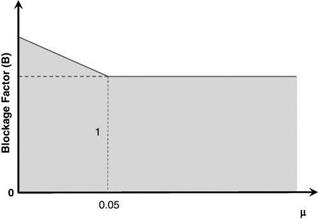
Figure A.2 Variation of blockage factor |
opposition to the respective rotor thrust directions. Therefore, in order to achieve the required component of force from either rotor, the thrust must exceed this by an amount equal to the download on the fuselage or fin. As the effect of these downwashes on the rotors will be altered by the superimposing of the forward flight velocity, the blockage effect will diminish with an increase in this forward flight velocity. In essence, the rotor downwash is carried increasingly downstream of the fuselage/fin, eventually causing no real fuselage/fin download from the main/tail rotor wake.
The application of this rotor blockage is to use a factor which multiplies the desired net thrust to account for the loss. As the forward velocity of the helicopter increases, the blockage factor will reduce from its specified hover value to unity. The variation is specified in a simple manner and for this example is based on the respective advance ratio. The blockage value refers to the hover condition, where the interaction with the fuselage/fin is greatest, and linearly decreases to unity at an advance ratio of 0.05, remaining at unity for higher advance ratios. This is illustrated in Figure A.2.
(Note the inclusion of the blockage factor BT for the tail rotor.)
The determination of the induced velocity of the tail rotor is the next part of the calculation. The advanced ratio components together with the thrust coefficient of the tail rotor are now required:
|
V mxT = VTT |
(A. 16) |
|
mZT = q |
(A. 17) |
The tail rotor is only required to develop a thrust, normal to the helicopter’s centreline, so has no need for any disc tilt; in consequence the disc plane is assumed parallel to the flight path.
A.3.2.2 Calculate Tail Rotor Downwash
Using the same iterative method, the tail rotor downwash, 1iT, is then calculated.
A.3.2.3 Assemble Tail Rotor Powers
The tail rotor power components are now calculated. Induced:
![]() PiT — kix ■ TT ■ Vtt ■ liT
PiT — kix ■ TT ■ Vtt ■ liT
Profile:
Total:
Ptott — PiT + Ppt (A. 20)
(Note that there is no parasite power for the tail rotor as the main rotor is assumed to be responsible for overcoming the parasite drag of the aircraft.)
A.3.3 Complete Aircraft
The total power required is now – calculated by summing the total powers for the main and tail rotors together, to which is added the power necessary to drive any auxiliary services (PAUX) such as oil pumps and electrical generators. It is to be expected that some losses will occur in the transmission and, to account for this, a factor is applied giving the power required from the engines as follows.
With the advance ratio components evaluated, the main rotor downwash can now be calculated using the iterative technique described in an earlier chapter:
A good starting value, for the iteration, is that for hover, namely:
![]() Ai OLD — 2^/~Ct
Ai OLD — 2^/~Ct
This now determines the downwash AiM.
A.3.1.3 Assemble Main Rotor Powers
The main rotor power components can now be calculated. Induced (note that the induced power factor kiM is included):
![]() PiM = kiM • Tm • VTM • ^iM
PiM = kiM • Tm • VTM • ^iM
Profile:
Parasite:
![]()
![]() PpARAM = D • V
PpARAM = D • V
Summing for the total:
Ptot M = PiM + Ppm + Pparam
A.3.2 Tail Rotor
The main rotor torque is now obtained from the total main rotor power, from which the tail rotor thrust value necessary for torque balance is calculated.
A.3.1.1 Calculate Main Rotor Thrust and Disc Attitude
The force balance diagram for the main rotor is shown in Figure A.1.
Resolving vertically:
Tcos(gS) – W (A.2)
Resolving horizontally:
 |
Tsin(gS) – D (A.3)
Figure A.1
From these we obtain for the disc tilt:
gS = tan_1(W) (A-4)
The main rotor thrust, with the application of blockage, becomes:
T — Bm VW2 + D2 (A.5)
Rotor blockage represents the download on the fuselage due to the rotor downwash and is applied to the main rotor thrust as a multiplying factor using the Bm factor.
The induced velocity of the main rotor can now be determined. Since actuator disc theory is being used, the advance ratio components parallel to and normal to the main rotor disc plane are needed together with the thrust coefficient.
The advance ratio is defined by:
Resolving parallel to the rotor disc:
![]()
![]() mXM = mM cos(gS)
mXM = mM cos(gS)
Resolving perpendicular to the rotor:
mZM — mM sin(gS)
The nomenclature used in the following sections is presented in Tables A.1 and A.2.
A.3 Overall Aircraft
The initial calculation is of the helicopter drag which, together with the weight, will allow the thrust and forward tilt of the main rotor to be determined.
|
Table A.1 Rotor
|
|
Drag @100 velocity units |
D100 |
|
Auxiliary power |
Paux |
|
Transmission loss factor |
TRLF |
|
Helicopter weight |
W |
|
Helicopter drag |
D |
|
Table A.2 Overall helicopter |
Drag can be specified in several ways; however, the method described here uses the drag force at a reference speed of 100 units (D100) at ISA sea-level air density as a basis. (This calculation can be readily adapted to any other specification of drag.) The drag of the helicopter is then calculated by factoring the D100 value with the square of the forward speed and linearly with respect to the air density, as follows:
s (A1)