Category COMPUTATIONAL AEROACOUSTICS

Three sample programs are provided in this appendix. The first set of programs is for solving the one-dimensional convective wave equation. There are two programs. The first program uses the DRP scheme. The second program uses the standard 2nd, 4th and 6th order central difference scheme for spatial discretization and the Runge-Kutta scheme for time marching. The second set of programs is for solving the linearized two-dimensional Euler equations. The DRP scheme is used. The third set of programs is for solving the non-linear three-dimensional Euler equations. The DRP scheme is used.

G.1 Sample Program for Solving the One-Dimensional Convective Wave Equation

The numerical solution to the following problem in an infinite domain is considered. The convective equation in dimensionless form is

d u d u

+ = 0 91 dx

Two types of initial conditions are used in this example

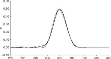
1. A Gaussian function.

2. A box car function i. e.,

u(x, 0) = H(x + L) – H(x – L) where H (x) is the unit step function.

The Fortran 90 program below computes the solution using the DRP scheme.

program DRP_1D

This code solves the 1-D convective wave equation on the real line using the DRP scheme

-equation is non-dimensionalized by mesh spacing and wave speed

-equation is discretized with 7-point spatial stencils and 4 level multi-step time advancement

-the solution is advanced from the initial conditions to the desired time and then output to file

Variables:

id – number of mesh points to the left and right of origin nmax – maximum number of time steps t – time

delt – time step u – solution values

k – time derivatives, dudt, at different time levels

kl – converts time level to index in k array a – spatial stencil coefficients

b – multi-step advancement coefficients

implicit none

integer, parameter::rkind=8,id=800 integer::n, l,nmax, bh integer, dimension(-3:0)::kl real(kind=rkind)::delt, h,t real(kind=rkind), dimension(-id-3:id+3)::u real(kind=rkind), dimension(-3:0,-id:id)::k real(kind=rkind), dimension(-3:3)::a real(kind=rkind), dimension(-3:0)::b integer::outdata=20 !

! Open output data file ‘out. dat’

!

open(unit=outdata, file="outDRP. dat", status="replace") !

! Optimized 7-point spatial stencil

!

a(-3)=-0.02003774846106832_rkind

a(-2)=0.163484327177606692_rkind

a(-1)=-0.766855408972008323_rkind

a(0)=0.0_rkind

a(1)=0.766855408972008323_rkind

a(2)=-0.163484327177606692_rkind

a(3)=0.02003774846106832_rkind

!

! Optimized multi-step

!

b(0)=2.3025580888_rkind

b(-1)=-2.4910075998_rkind

b(-2)=1.5743409332_rkind

b(-3)=-0.3858914222_rkind

I

! Set simulation parameters I

delt=0.1_rkind! time step size (stability/accuracy limit is 0.2111) nmax=3000 ! maximum number of time steps I

! Set ‘boundary’ conditions (assume u=0 far from origin)

I

u(-id-3)=0.0_rkind

u(-id-2)=0.0_rkind

u(-id-1)=0.0_rkind

u(id+1)=0.0_rkind

u(id+1)=0.0_rkind

u(id+3)=0.0_rkind

!

! Set initial conditions!

t=0.0_rkind

!

! Gaussian function with half-width ‘bh’ and height ‘h’ !bh=3

!h=0.5_rkind! do l=-id, id

! u(l)=h*exp(-log(2.0_rkind)*(real(l, rkind)/real(bh, rkind))**2) !end do!

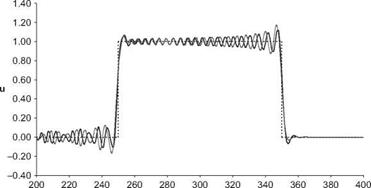
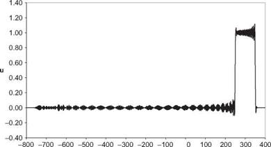
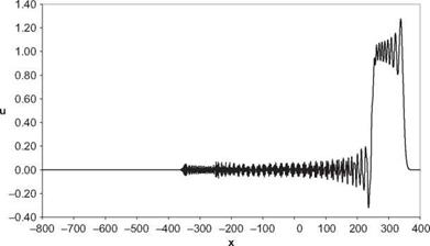
! Boxcar

!

u=0.0_rkind

u(-50:50)=1.0_rkind

!

! Set solution to zero for t<0

!

k=0.0_rkind

kl(-3)=-3

kl(-2)=-2

kl(-1)=-1

kl(0)=0

!

!——————————————————————

!

! Main loop – march nmax steps with multi-level DRP

do n=1,nmax!

t=t+delt

write (*,*)"n: ",n," t: ",real(t,4)

!

! Update k

!

do l=-id, id

k(kl(0),l)=a(-3)*u(l-3)+a(-2)*u(l-2)+a(-1)*u(l-1)+a(1)*u(l+1)+a(2)*u(l+2)+a(3)*u(l+3) end do!

! Update u to time level n

!

do l=-id, id

u(l)=u(l)-delt*(b(0)*k(kl(0),l)+b(-1)*k(kl(-1),l)+b(-2)*k(kl(-2),l)+b(-3)*k(kl(-3),l)) end do!

! Shift k array back kl =cshift(kl,1)

end do!

! Output u results !

50 format(i8,e16.7e3) do l=-id, id

write (outdata,50)l, u(l) end do!

stop

end program DRP_1D

The Fortran 90 program below computes the solution to the convective wave equa­tion by means of the standard 2nd, 4th and 6th order central difference scheme for spatial discretization and the Runge-Kutta scheme for time marching.

program RK4_1D

This code solves the 1-D convective wave equation on the real line using the standard fourth order Runge-Kutta scheme – equation is non-dimensionalized by mesh spacing and wave speed

-equation can be discretized with either 6th,4th,2nd order spatial stencils

-the solution is advanced from the initial conditions to the desired time and then output to file

Variables:

id – number of mesh points to the left and right of origin nmax – maximum number of time steps t -time delt – time step

и, ut – solution values

к, k1,k2 – time derivatives, dudt

a2	-2nd	order	spatial	stencil	coefficients
a4	-4th	order	spatial	stencil	coefficients
a6	-6th	order	spatial	stencil	coefficients

implicit none

integer, parameter::rkind=8,id=800 integer::n, l,nmax, bh, iorder real(kind=rkind)::delt, dth, dt6,h, t real(kind=rkind), dimension(-id-3:id+3)::u, ut real(kind=rkind), dimension(-id:id)::k, k1,k2 real(kind=rkind), dimension(-1:1)::a2 real(kind=rkind), dimension(-2:2)::a4 real(kind=rkind), dimension(-3:3)::a6 integer::outdata=20 !

! Open output data file ‘out. dat’

!

open(unit=outdata, file="outRK4.dat", status="replace") !

! 2nd order spatial stencil

!

a2(-1)=-0.5_rkind

a2(0)=0.0_rkind

a2(1)=0.5_rkind

!

! 4th order spatial stencil

!

a4(-2)=1.0_rkind/12.0_rkind

a4(-1)=-2.0_rkind/3.0_rkind

a4(0)=0.0_rkind

a4(1)=2.0_rkind/3.0_rkind

a4(2)=-1.0_rkind/12.0_rkind

6th order stencil

a6(-3)=-1.0_rkind/60.0_rkind

a6(-2)=3.0_rkind/20.0_rkind

a6(-1)=-3.0_rkind/4.0_rkind

a6(0)=0.0_rkind

a6(1)=3.0_rkind/4.0_rkind

a6(2)=-3.0_rkind/20.0_rkind

a6(3)=1.0_rkind/60.0_rkind

!

! Set simulation parameters!

delt=0.4_rkind! time step size

dth=delt*0.5_rkind

dt6=delt/6.0_rkind

nmax=750 ! maximum number of time steps iorder=6 ! order of the spatial stencil (2,4,6)

!

! Set ‘boundary’ conditions (assume u=0 far from origin) !

u(-id-3)=0.0_rkind

u(-id-2)=0.0_rkind

u(-id-1)=0.0_rkind

u(id+1)=0.0_rkind

u(id+1)=0.0_rkind

u(id+3)=0.0_rkind

!

ut=0.0_rkind

!

! Set initial conditions!

t=0.0_rkind

!

! Gaussian function with half-width ‘bh’ and height ‘h’ !bh=3

!h=0.5_rkind! do l=-id, id

! u(l)=h*exp(-log(2.0_rkind)*(real(l, rkind)/real(bh, rkind))**2) !end do!

! Boxcar!

u=0.0_rkind

u(-50:50)=1.0_rkind

Initial du/dt

call dudt(u, k,iorder)

!

!………………………………………………………….

!

! Main loop – march nmax steps in time using RK4 integration!

do n=1,nmax!

t=t+delt

write (*,*)”n: ",n," t: M, real(t,4)

!

! Second step!

do l=-id, id ut(l)=u(l)+dth*k(l) end do

call dudt(ut, k1,iorder)

!

! Third step

!

do l=-id, id ut(l)=u(l)+dth*k1(l) end do

call dudt(ut, k2,iorder)

!

! Fourth step

!

do l=-id, id ut(l)=u(l)+delt*k2(l) k2(l)=k2(l)+k1(l) end do

call dudt(ut, k1,iorder)

!

! Update u

!

do l=-id, id

u(l)=u(l)+dt6*(k(l)+k1(l)+2.0_rkind*k2(l)) end do!

! Update dudt

!

call dudt(u, k,iorder) end do

! Output u results I

50 format(i8,e16.7e3) do l=-id, id

write (outdata,50)l, u(l) end do!

stop

!

contains

!

subroutine dudt(f, kf, iflag) !

!

! Calculate the derivative du/dt=-du/dx of the convectice wave eqn! – iflag is a flag for the spatial stencil (2nd,4th,6th order)

!

!

implicit none

integer, intent(in)::iflag

real(kind=rkind), intent(in), dimension(-id-3:id+3)::f real(kind=rkind), intent(out), dimension(-id:id)::kf integer::l!

select case (iflag) case (2) do l =-id, id

kf(l)=-(a2(-1)*f(l-1)+a2(1)*f(l+1)) end do case (4) do l =-id, id

kf(l)=-(a4(-2)*f(l-2)+a4(-1)*f(l-1)+a4(1)*f(l+1)+a4(2)*f(l+2)) end do case (6) do l =-id, id

kf(l)=-(a6(-3)*f(l-3)+a6(-2)*f(l-2)+a6(-1)*f(l-1)+a6(1)*f(l+1)+a6(2)*f(l+2)+a6(3)*f(l+3)) end do end select!

return

end subroutine dudt !

end program RK4_1D

Samples of computed results and the exact solutions are shown below.

Gaussian, t=300 I—— DRP ——- RK4-6th……… Exact | x

Boxcar, t=300 I—— DRP RK4-6th……………… Exact |

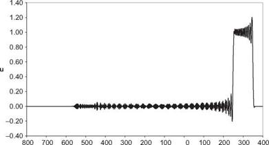
Boxcar, t=300, DRP Scheme x

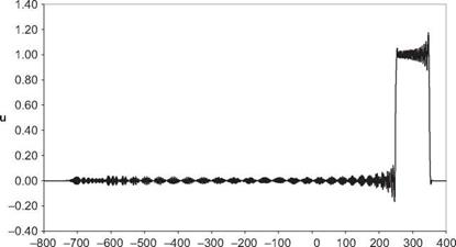
Boxcar, t=300, RK4-2nd

Boxcar, t=300, RK4-6th x

1.1. The governing equation and boundary conditions for a rectangular vibrating membrane of width W and breadth B are

92U 2 / d2Ы d2U

dt2 dx2^~ dy2

At x = 0, x = W, y = 0, y = B, u = 0,

where U is the displacement of the membrane. It is easy to show that the normal mode frequencies of the vibrating membrane are

[2]/2

, where j and к are integers.

Now divide the width into N subdivisions and the breadth into M subdivisions so that Ax = W/N and Ay = B/M. Suppose a second-order central difference is used to approximate the x and y derivatives. This converts the partial differential equation into a partial difference equation, as follows:

[3]

The conditions for E to be a minimum are

[4] For convenience, D(a Ax) may be normalized so that

D (n) = 1. (7.18)

The right side of Eq. (7.14) is a truncated Fourier cosine series. To ensure that D (a Ax) is small when a Ax is small but becomes large when a Ax ^ n, one may use a Gaussian function centered at a Ax = n with half-width a as a template for choosing the Fourier coefficients d. This is done by determining dj such that the integral

[5] There should be no damping for long waves. That is, D (a Ax) ^ 0 as aAx^0. This requires

3

d0 + 2 dj = 0. (7.17)

j=1

7.1. Let us reconsider the initial value problem

9 u d u

+ = 0 9t dx

t = 0, u = H (x + 50) – H (x – 50), where H (x) is the unit step function.

Compute the solution using the 7-point DRP scheme with artificial selective damping. Use a At that satisfies the numerical stability requirement.

[7] Use RA = 0.3, where Ra is the artificial mesh Reynolds number.

[8] Use RA = 0.3/At.

Plot u(x, t) at t = 300 for each case.

7.2. Real fluids have molecular viscosity that tends to damp out long and short wave disturbances. This problem focuses on how best to compute viscous terms to simulate real viscous effects. At the same time, it provides an example illustrating why

[9] Use RA = 3.

[10] 3

— aj ФJ.

Ді j j

j=-3

[11]+dMA)U+A і+(1 – m2 ) 2 ВI=<9-38)

where u(x, y, t) = U(x, y)e-1 ®f.

The second step is to introduce damping into the equation through a so-called complex change of variables. Let о x(x) > 0, о (y) > 0 be the absorption coefficients. The complex change of variables is to let

9.1. Many aeroacoustic problems involve the scattering of vorticity or acoustic waves by an object. To simulate this class of problems in the time domain, the incoming waves are generated by the boundary conditions imposed on the artificial external boundaries of the computation domain.

Dimensionless variables with respect to length scale L (L will be chosen later), velocity scale aTO (ambient sound speed), time scale L/aTO, density scale pTO (ambient density), and pressure scale p^a^ are used. Suppose there is a uniform mean flow

11.1. The optimized extrapolation method can be applied even when the stencil points are not spaced uniformly apart. Let the coordinates of the stencil points be x0, x_1, x_2,…, x__7 (a 7-point stencil). Suppose the extrapolation point is at x = x0 + n. The extrapolation formula is

[14]

f (x0 + n) = Y^ Sjf(x- j )•

j=0

[15]

[16] (R, в, ф, ю)

[17] 0 < r < 0.8

where x (ш) is a random-phase function, a0 is the speed of sound, and А(ш) is the amplitude function.

For numerical computation, the spectrum S(ш) has to be discretized. A simple way is to divide the spectrum into narrow bands with bandwidth Дшj for the jth band. The bandwidths need not be constant. Let the center frequency of the jth band be ш j. To avoid harmonic interaction, it will be required that no center frequency is the harmonic of another, i. e., ojj = Кшк, j = k, K = integer.

A spectrum is a distribution of acoustic energy with respect to frequency. The energy in the jth band is S(oij )Дш j as Дш j ^ 0. Now, for small Дш j, a reasonable approximation is to assume that the energy in the jth band is concentrated in the center frequency шj. That is, the jth band is approximated by a single wave in the following form:

A more formal way of stating the approximation is to replace the amplitude function А(ш) of Eq. (F1) by a row of delta functions, i. e.,

TO

А(ш) = ^2, Aj8(ш — шj) (F2)

j=—TO

The energy of a discrete frequency wave is equal to 1 Ajj. Thus, to conserve energy, it is necessary to require

2 Aj = S(ш)Дш j.

where xj is a random number, specifically x-j = xj.

Now, the two-point space-time correlation function of the sound wave field given by Eq. (F4) is

p(x’, t’)p(x", t’ + t)

NN

= 2[S(“j)S(rnk)A<»j A“] ^

(F5)

where the overbar denotes a time average. Consider, for the moment, the time – averaged terms on the right side of Eq. (F5).

This time average is equal to zero except when k = j. In this special case, by expanding the second cosine term on the right side by compound angle formula, it is readily found that

where 5 jk is the Kronecker delta. Therefore, Eq. (F5) reduces to

The autocorrelation function of the wave field may be found by setting x" = x’ in Eq. (F7). This yields

N

p(x’, t’)p(x’, t’ + t) = ^2 S(«k)A«k cos(«kT).

k=—N

The power of the acoustic field is given by setting T = 0. Thus,

_______ N ^

p2 (x’, t) = E S(rnk)A«k ^ / S(«)d«; in the limit A«k ^ 0. (F9)

U Л Г *

Eq. (F9) indicates that S(«) is the spectrum of the wave field.

Another way to find the spectrum is to make use of the fact that the spectrum is the Fourier transform of the autocorrelation function. That is, if S(«) is the spectrum of the wave field given by Eq. (F4), then it is equal to the Fourier transform of the right side of Eq. (F8) as follows:

L N

— 1C N

S(«) = — I ^2 S(«k)A«kcos(«kT)e’«TdT.

Ж-L k=-N

In the limit A«k ^ 0,

L L

S(«) = 2П // S(Q) cos(^T)e’«T dT dQ,

1

= 2[S(«) + S(-«)] = S(«).

The usual symmetry assumption, i. e., S(-«) = S(«) is assumed here.

A special case of interest is the sound field associated with a broadband monopole source. Let (У, в,ф) be the spherical coordinates system centered at the monopole. Y is the radial coordinate (see Figure 14.12). The sound field according to the energy conserving discretization procedure is

In many aeroacoustics problems, it is sometimes advantageous to compute the mean flow first and then to turn the noise sources on and compute the sound field using the same computer code. This becomes a necessity if the sound intensity is very low; smaller than the error of the numerical mean flow solution (in comparison with the exact solution). One drawback of this approach is that it could take a long time to converge to a steady state when using an almost nondissipative computation scheme such as the dispersion-relation-preserving (DRP) scheme. On the other hand, using a more dissipative scheme might damp out the sound. Because of the nearly nondis­sipative nature of the scheme, the only way by which the residual associated with the initial condition can be reduced to a very low level is to have it expelled slowly through the boundaries of the computational domain. This sometimes could take a very long computation time. A method to achieve accelerated convergence to steady state without compromising accuracy would, therefore, be very useful.

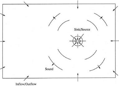
To illustrate a way to attain accelerated convergence to steady state, consider a two-part problem of computing the mean flow created by a localized sink/source and then the sound field created by tiny oscillations of the sink/source strength. The problem is as shown in Figure E1. In two dimensions, the governing equations are as follows:

Figure E1. Acoustic radiation from an oscillatory sink/source flow.

In Eq. (E5) (x0, y0) are the coordinates of the center of the sink/source. Nondi­mensional variables with a0 (sound speed) as the velocity scale, Ax as the length scale, Ax/a0 as the time scale, p0 as the density scale, and p0a0 as the pressure scale are used in all computations.

In this illustration, the computational domain of Figure E1 is discretized by using a square mesh with Ax = Ay. A120 x 100 computational grid centered at the origin of coordinates is used. The following values are assigned to the source parameters:

a = І36:, r0 = 12, Q = 0.0456, x0 = 20, y0 = 0.

To start the mean flow computation, a zero initial condition is used. The solution is time marched to a steady state by means of the 7-point stencil DRP scheme. Artificial selective damping with a mesh Reynolds number (RAx = a°7^) equal to

a

10 is added to the discretized equations. With such a small amount of damping, in a trial computation, the residual is able to settle down over time to a magnitude of the order of 10-13 (the residual is effectively the value of the time derivative or its finite difference approximation). This is just the machine truncation accuracy (single precision). This very low background noise level is, however, a necessary condition for performing the subsequent computation of the very low intensity sound (of the order of 10-10) produced by extremely tiny oscillations of the sink/source strength.

Through numerical experimentation, the following technique referred to as the “canceling the residuals” has been found to be very effective in promoting acceler­ated convergence. Since the difference between the numerical and the exact solution is of the order of a percent, further time marching calculation is a waste of effort in terms of improving the accuracy of the numerical solution, once the residuals reach a level of order 10-5. With this in mind, it is possible to add terms that are exactly equal in magnitude, but opposite in sign to the residuals to the right side of

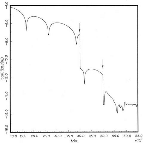
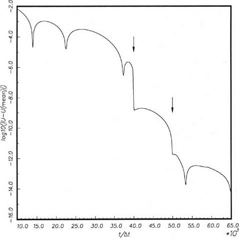
Figure E2. Time history of the residual of the м-velocity component at the grid point (-20, -25). Arrows indicate the application of the canceling-the-residuals technique for accelerated convergence.

each of the governing equation. These are terms of order 10-5 or less and would, therefore, not materially affect the accuracy of the steady-state numerical solution. The added terms may be regarded as minute artificial distributed sources of fluid, momentum, or heat. The consequence of adding these minute source terms is to render the residuals instantaneously to zero. Of course, for a multilevel marching scheme, the residuals of the scheme are greatly reduced in this way, but they would not be exactly equal to zero at the next time level. Numerical experiments indicate that when this canceling-the-residuals procedure is performed, the overall residual of the computation drops almost instantaneously by several orders of magnitude. This method can be applied repeatedly until machine accuracy is achieved.

Figure E2 shows the time history of the residual, log10 | d |, at the point (-20,-25). The arrows in this figure indicate when the canceling-the-residuals tech­nique is applied. It is clear that there is a dramatic decrease (of 3 to 4 orders of magnitude) in the residual immediately after each application of the method.

Figure E3. Convergence history of the м-velocity component at the point (+20, -25). Arrows indicate the application of the canceling-the-residuals technique for accelerated convergence.

Figure E3 shows the corresponding convergence history of the м-velocity compo­nent at the mesh point (+20, -25). The computed solution rapidly approaches the eventual mean value of the velocity component right after each application of the accelerated convergence technique. It is worthwhile to mention that the method works in all the cases that have been tested. The total computer run time needed to attain a steady-state numerical solution is drastically reduced in each instance.

The dispersion-relation-preserving (DRP) scheme is well suited to compute numeri­cal solutions of diffusion equations. To illustrate this, consider computing the solution of the initial value problem governed by the heat equation as follows:

дU f д2U д2u

dt д X2 + д y2

at t = 0, u = f (x, y).

Before implementing the DRP scheme, it is advantageous to cast (D1) into a system of first-order equations. This may be done by introducing two auxiliary variables defined by

(D1) becomes

д U / д V д W дt дX^~ ду2

Now, the system of equations (D3) to (D5) is equivalent to (D1).

Upon applying the DRP scheme to (D3) to (D5), the finite difference system is

1 3 v(n) = — a U(n) Vl, m = Дх ajUl+j, m	(D6)
j=-3
13 W(n) = 1 a U(n) Wl, m = Ду ajUl, m+j y j=-3	(D7)
E(n) = K h a 1 v(n) i 1 w(n) lm =-3 aj AxVl+j, m + AyWlm+j	(D8)
3 u’,t=um+it c bjE’m j	(D9)
j=0

The time step At that can be used in (D9) is constrained by stability considera­tion. To determine the largest time step without triggering numerical instability, the first step is to find the dispersion relation of the system of finite difference equations (D6) to (D9). This is done by generalizing the discretized system to a set of finite difference equations with continuous variables and then take their Fourier-Laplace transforms. This leads to (a Ф will be used to denote the Fourier-Laplace transform of Ф ) the following:

v — iaU	(D10)
w — ів U	(D11)
Ё — K(iav + івії)	(D12)
— f(a^) p -і(&Н————- — Ё, 2n	(D13)

where f (a, в) is the Fourier transform of the initial condition f(x, y). a and в are the Fourier transform variables in the x and y directions, and ы is the Laplace transform variable. The solution of (D10) to (D13) is

і f (а, в)

U — 2 ♦

2п ы + ік (a2 + в )

The dispersion relation is given by setting the denominator of (D14) to zero, i. e.,

ы — – ік(а2 + в2). (D15)

Note that ы is purely imaginary for real a and в. According to the stability dia­gram of the DRP scheme (Figure 3.2) the stability limit along the negative imaginary axis of the rnAt plane is &At | < 0.29 . Thus, by dispersion relation (D15), in order to maintain numerical stability, it is required that

к(а2 + в2 )At < 0.29. (D16)

(D16) may be rewritten as

For the 7-point stencil DRP scheme, a Ax and в Ay are less than 1.75. Thus, by replacing a Ax and в Ay by 1.75 in (D17), the largest permissible time step, AtMax, is given by

It is a fact that diffusion current always flows outward from the source. Math­ematically speaking, this means that the solution at a point, away from the source depends only on the solution at points closer to the source. Therefore, at the bound­ary of a finite computation domain, the appropriate boundary treatment is to use backward difference stencils in the boundary region. There is no need to impose special boundary conditions.

As a simple numerical example, consider the case of an initial Gaussian pulse,

i. e.,

where b is the half-width of the pulse. The exact solution is

Figure D1 shows the result of a computation using the 7-point stencil DRP scheme for the case b = 3. The length scale is Ax = Ay. The time scale is x^ . A 100 x 100 mesh was used in the computation. The numerical solutions at t = 20, 40, 80, 160, and 300 are displayed in the figure. The exact solution is shown by a dotted line. However, it cannot be easily seen because it differs from the numerical solution by less than the thickness of the lines of the figure. The numerical solution is extremely accurate.

The one-dimensional continuity, momentum, and energy equations of a compress­ible, inviscid fluids are

dp dp du

dt 9x H 9x

9 u 9 u 1 9 p

+ u + — 0

dt dx p dx

9p 9p du

+ u + у p — 0. dt 9 x 9 x

This system of three equations supports three sets of characteristics. These characteristics may be found by combining the three equations in a special way. For this purpose, multiply (C1) by X and (C2) by в and add to (C3), where X and в are functions of the dependent variables p, u, and p.

Now X and в may be chosen such that all the derivatives of the dependent variables are in the form of a common convective derivative as follows:

— + V—. dt dx

There are three possible choices. They are

1. в — 0, X — – .

p

In this case, (C4) becomes

dp dp y p 9p 9p

+ u — + u — 0.

dt 9 x p dt 9 x,

Now, in the x-t plane, along the curve

dx

— u, dt

d — YP 0? = 0, (C7)

dt p at

where

d d dx d d d

dt dt + dt dX dt + U dX

along the P-characteristic. (C7) may be expressed in a differential form as follows:

dp — — dp = 0. (C8)

p

This may be integrated to yield

d( — ) = 0 or — = constant along a P-characteristic. (C9)

PV Pv

In other words, the flow is isentropic following the motion of a fluid element.

2. X = 0, в = P (—^ = pa

d— dU

— + p a— = 0 or dp + padu = 0. dt dt

Consider evaluating the following integral in the limit X ^ ro.

b

1,X) = и, х)е"»<Ъ.

a

It was pointed out by Lord Kelvin (1887) that for large X the function еіЛФ(х) will oscillate wildly with almost complete cancellation. Significant contribution to the integral comes from small intervals of х where Ф(х) varies slowly. This happens when Ф'(х) = 0 or at the stationary points of Ф(х).

Suppose Ф(х) has only one stationary point in (a, b), say at х = с. That is

Ф/;, с)

Ф, х) = Ф, с) +—— 2C, х – c2 ) + •••• (B2)

Since the major contribution to (B1) comes around х = с, asymptotically the integral is given by

C+S

И, с)е1ХФ, с) еФ" ,c),x-c)2Dx.

с—S

It is possible to change the limits of integration to – ro to ro as the error of extend­ing 5 to ro is asymptotically small (nearly complete cancellation). On accounting for that Ф"(с) may be positive or negative, the integral of (B3) may be evaluated to give

b 1

lim И, х)еаФ, х)ёх – — 2 И, cyH(c)+sgn^"(c))f], (B4)

x->ro w X Ф, c)| w ()

a

where sgn( ) is the sign of ( ).

A.1 Fourier Transform

Let f(x) be an absolutely integratable function; i. e., f—°TO F(x)dx < to, then F(x) and its Fourier transform F(a) are related by

TO to

F(a) = j F(x)e—laxdx, F(x) = j F(a)eiaxda.

— TO —TO

Derivative Theorem

By means of integration by parts, it is easy to find

TO TO

d F 1 d F la

— = — —e—laxdx = — F (x)e—laxdx = laF (a).

dx 2n dx 2n

— TO —TO

Shifting Theorem

TO

F(x + X)e—laxdx = 2^ j F(n)e—lan+laXdn = elaXF(a).

— TO

A.2 Laplace Transform

Let f(t) satisfy the boundedness condition /TO e—ct f (t)dt < to for some c > 0, then f(t) and its Laplace transform f(^) are related by

TO

f(oi) = 2П J f (t)elmtdt, f (t) = 2П J f (M)e—lmtdrn.

0 г

The inverse contour г is to be placed on the upper-half «-plane above all poles and singularities of the integrand (see Figure A1). This condition is necessary in order to satisfy causality.

Figure Al. Complex «-plane showing the inverse contour Г, • poles, ~~~~ branch cut.

Derivative Theorem

By applying integration by parts to the integral below, it is straightforward to show

Shifting Theorem

Let the initial conditions be

Ф, 0 < t < X 0, t < 0

then,

о о f(t + X _ 21 f f (t + X)eilotdt _ 2^ j f (nV^-^dn 0 X Г X 1 e~i«X f(v) – 2nj f (n)eiandn _ ^— f(v) + (1 – eicoX) 2п Ш 0

Similarly,

f(t – X _ eiaX f(co).

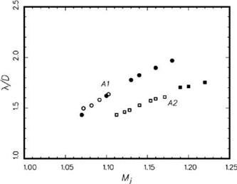
It is well known that at low supersonic jet Mach numbers, there are two axisymmetric screech modes. They are referred to as the A1 and A2 modes. Earlier, Norum (1983) had compared the frequencies of the A1 and A2 modes measured by a number of investigators. His comparison indicated that the screech frequencies and the Mach number at which transition from one mode to the other takes place (staging) could vary slightly from experiment to experiment. Experimentalists generally agree that

Figure 15.58. Comparison between acoustic wavelengths of simulated screech phenomenon and the experimental measurements of Ponton and Seiner (1992). o, □, Measurements; •, ■, simulations.

the screech phenomenon is extremely sensitive to minor details of the experimental facility and jet operation conditions.

By using this numerical method, it is found that numerical simulation does reproduce both the A1 and the A2 axisymmetric screech modes. Figure 15.58 shows the variation of the computed X/D, where X is the acoustic wavelength of the tone,

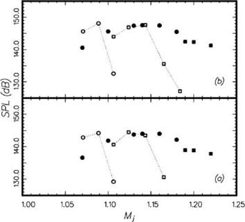
Figure 15.59. Intensity of axisymmetric jet screech tones at the nozzle exit plane. (a) r/D = 0.889, (b) r/D = 0.642. Experiment (Ponton and Seiner, 1992): o, A1 mode; □, A2 mode. Numerical simulation: •, A1 mode; ■, A2 mode.

with jet Mach number. Since X/D = aTO/( fD) , where f is the screech frequency, this figure essentially provides the tone frequency Mach number relation. Plotted on this figure also are the measurements of Ponton and Seiner (1992). The data from both the numerical simulation and experiment fall on the same two curves, one for the A1 mode and the other for the A2 mode. This suggests that the computed screech frequencies are in good agreement with experimental measurements. This is so, although the staging Mach number is not the same.

Ponton and Seiner (1992) mounted two pressure transducers at a radial distance of 0.642D and 0.889D, respectively, on the surface of the nozzle lip in their exper­iment. By means of these transducers, they were able to measure the intensities of screech tones. Their measured values are plotted in Figure 15.59. The transducer of Figure 15.59b is closer to the jet axis and, hence, shows a higher decibel level. Plotted on these figures also are the corresponding tone intensities measured in the numerical simulation. The peak levels of both physical and numerical experiments are nearly equal. Thus, except for the difference in the staging Mach number, the numerical simulation is, indeed, capable of providing accurate screech tone intensity prediction as well.

It has been found that numerical algorithm described above is capable of reproduc­ing the jet screech phenomenon computationally. The nozzle configuration in the experiment of Ponton and Seiner (1992) is used in the simulation. Figure 15.55 shows the computed density field in the x-r plane at one instance after the initial transient disturbances have propagated out of the computational domain. The screech feed­back loop locks itself into a periodic cycle without external interference. As can be seen, sound waves of the screech tones are radiated out in a region around the fourth and fifth shock cell downstream of the nozzle exit. Most of the prominent features of the numerically simulated jet screech phenomenon are in good agreement with physical experiment.

15.6.2.1
Mean Velocity Profiles and Shock Cell Structure

To demonstrate that numerical simulation can, indeed, reproduce the physical exper­iment, the accuracy of the computed mean flow velocity profiles of the simulated jet is tested by comparison with experimental measurements. For this purpose, the time-averaged velocity profiles of the axial velocity of a Mach 1.2 cold jet from one jet diameter downstream of the nozzle exit to seven diameters downstream at one diameter intervals are measured from the numerical simulations. They are shown as a function of n* = (r – r05)/x in Figure 15.56, where r05 is the radial distance from the jet axis to the location where the axial velocity is equal to one half of the fully expanded jet velocity. Numerous experiments have shown that the mean velocity profile when plotted as a function of n* would nearly collapse into a single curve. The single curve is well represented by an error function in the following form:

U = 0.5[1 – erf (an*)], Uj

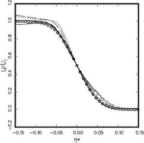Figure 15.56. Comparison between com­puted mean velocity profiles at M. = 1.2 and experiment (Lau, 1981). Simulation

results:——– , x/D = 1.0;——– , x/D =

2.0; — • —, x/D = 3.0;———– , x/D =

4.0;——— , x/D = 5.0;—– ,x/D = 6.0;

………… , x/D = 7.0. Experiment U/U. =

0.5[1 – erf(an*)]; o, a = 17.0.

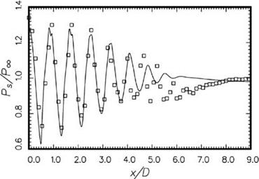
Figure 15.57. Comparison between calculated time-averaged pressure distribution along the centerline of a Mach 1.2 cold jet and the measurement of Norum and Brown (1993).- , simulation; □, experiment.

where a is the spreading parameter and Uj is the fully expanded jet exit velocity. Extensive jet mean velocity data had been measured by Lau (1981). By interpolating the data of Lau to Mach 1.2, it is found that experimentally a is nearly equal to 17.0. The empirical formula with a = 17.0 is also plotted in Figure 15.56 (the circles). It is clear that there is good agreement between measured mean velocity profile and those of the numerical simulation.

One important component of the screech feedback loop is the shock cell struc­ture inside the jet plume. To ensure that the simulated shock cells are the same as those in an actual experiment, the time-averaged pressure distribution along the centerline of the simulated jet at Mach 1.2 is compared with the experimental mea­surements of Norum and Brown (1993). Figure 15.57 is a plot of the simulated and measured pressure distribution as a function of downstream distance. It is clear from this figure that the first five shocks of the simulation are in good agreement with experimental measurements both in terms of shock cell spacing and amplitude. Beyond the fifth shock cell, the agreement is less good. However, it is known that screech tones are generated around the fourth shock cell. Therefore, any minor dis­crepancies downstream of the fifth shock cell would not invalidate the screech tone simulation.

The DRP scheme is a central difference scheme and, therefore, has no intrinsic dissipation. For the purpose of eliminating spurious short waves and to improve numerical stability, artificial selective damping terms are added to the discretized finite difference equations. For the present problem, artificial selective damping is also critically needed for shock-capturing purposes.

In the interior region, the 7-point damping stencil with a half-width of a = 0.2n is used. An inverse mesh Reynolds number (Яд[17] = va/(amAx)), where ua is the arti­ficial kinematic viscosity, of 0.05 is prescribed over the entire computation domain. This is to provide general background damping to eliminate possible propagating spurious waves. Near the boundaries of the computational domain where a 7-point stencil does not fit, the 5- and 3-point damping stencils given in Section 7.2 are used.

Spurious numerical waves are usually generated at the boundaries of a computa­tional domain. The boundaries are also favorite sites for the occurrence of numerical instability. This is true for both exterior and interior boundaries such as the nozzle walls and buffer regions where there is a change of mesh size. To suppress both the generation of spurious numerical waves and numerical instability, additional artificial selective damping is imposed along these boundaries. Along the inflow, radiation, and outflow boundaries, a distribution of inverse mesh Reynolds number in the form of a Gaussian function with a half-width of 4 mesh points (normal to the boundary) and a maximum value of 0.1 right at the outmost mesh points is incor­porated into the time marching scheme. Adjacent to the jet axis, a similar addition of artificial selective damping is implemented with a maximum value of the inverse mesh Reynolds number at the jet axis set equal to 0.35. On the nozzle wall, the use

of a maximum value of additional inverse mesh Reynolds number of 0.2 has been found to be very satisfactory.

The two sharp corners of the nozzle lip and the transition point between the use of the outflow and the radiation boundary condition on the right side of the computational domain are locations requiring stronger numerical damping. This is carried out by adding a Gaussian distribution of damping around these special points.

As shown in Figure 15.54, the four computational subdomains are separated by buffer regions. Here, additional artificial selective damping is added to the finite difference scheme. In the supersonic region downstream of the nozzle exit, a shock cell structure develops in the jet flow. In order to provide the DRP scheme with shock-capturing capability, the variable stencil Reynolds number method discussed in Section 8.3 is used. The jet mixing layer in this region has a very large velocity gradient in the radial direction. Because of this, the Ustencil of the variable stencil Reynolds number method is determined by searching over the 7-point stencil in the axial direction. In the radial direction only the 2 mesh points immediately adjacent to the computational point are included in the search. An inverse stencil mesh Reynolds number distribution of the following form:

4.5F (x)G(r),

where

1, 0 < x < 9

is used. It is possible to show, based on the damping curve (a = 0.3n), that the vari­able damping has minimal effect on the instability wave of the feedback loop. Also, extensive numerical experimentations indicate that the method used can, indeed, capture the shocks in the jet plume and that the time-averaged shock cell structure compares favorably with experimental measurements.