Our heavyweight helicopter equal in the world does not have
In Rostov started production of the most load-lifting rotary-wing car The Russian holding «Helicopt[...]

Everything about aircrafts and helicopters. News and events in aviation worldwide. Civil, transportation, military helicopters and airplanes.

Everything about aircrafts and helicopters. News and events in aviation worldwide. Civil, transportation, military helicopters and airplanes.

Everything about aircrafts and helicopters. News and events in aviation worldwide. Civil, transportation, military helicopters and airplanes.

Everything about aircrafts and helicopters. News and events in aviation worldwide. Civil, transportation, military helicopters and airplanes.


Regarding wing loading, although the overall correlation shown in Eq. (1-5) seems reasonable, Greenewalt [55] found that, in many cases, the relation between wing loading and mass increases more slowly than that indicated in Eq. (1-5). For example, the three families of birds (i. e., the Passeriforms, the Shorebirds, and the Ducks) do not follow the one-third law. As indicated in Table 1.3, for hummingbirds, wing loading is almost independent of body mass; hence different species can have the same wing loading. Tennekes [29] used the data collected by Greenewalt [55] and summarized the various scaling relations for seabirds, shown in Table 1.4. All gulls and their relatives have long, slender wings and streamlined bodies, so it was reasonable to assume geometric similarity. From Table 1.4 it is obvious that the wing loading and cruising speed generally increase with weight.
1.2.4 Aspect Ratio
As for aircraft, the aspect ratio (AR) can give an indication of the flight characteristics for flapping animals. The AR is a relation between the wingspan b and the wing area S:
b2
AR = j. (1-7)
[4] When the AoA is increased (from 4.03° to 7.82°), the adverse pressure gradient on the upper surface grows, which intensifies the Tollmien-Schlichting (TS) wave, resulting in an expedited laminar-turbulent transition process. A shorter LSB leads to more airfoil surface being covered by the attached turbulent boundary-layer flow, resulting in a lower drag. This corresponds to the lift-drag polar’s left turn.
[5] At a lower AoA, for example, 2.75°, there is a long bubble on the airfoil surface, which leads to a large drag.
![]() Scaling laws have clearly established that MAVs and small natural flyers cannot operate with the same lift and thrust generation mechanisms as larger aircraft and that moving wings are needed to conduct the flight mission. Furthermore, these flyers can substantially benefit from active and passive morphing for flight performance enhancement and control, just like the flyers that we see in nature. For example, Lee et al. [530] investigated longitudinal flight dynamics of a bio-inspired ornithopter with a reduced-order aerodynamics model, including wing flexibility effects. They showed that this ornithopter is robust to external disturbances due to its trimmed flight dynamic characteristics that limit cycle oscillation. Furthermore the mean forward flight speed increases almost linearly with the flapping frequency. Inspiration from nature will give us insight on how to manage the complex flight environment. Still we need to keep in mind there is no single perfect mechanism that all flyers should adopt. It is ultimately up to the scientists and engineers to figure out the best combination of the available techniques for a given flyer to suit its size, weight, shape, and flight environment, including wind gust, and mission characteristics.
Scaling laws have clearly established that MAVs and small natural flyers cannot operate with the same lift and thrust generation mechanisms as larger aircraft and that moving wings are needed to conduct the flight mission. Furthermore, these flyers can substantially benefit from active and passive morphing for flight performance enhancement and control, just like the flyers that we see in nature. For example, Lee et al. [530] investigated longitudinal flight dynamics of a bio-inspired ornithopter with a reduced-order aerodynamics model, including wing flexibility effects. They showed that this ornithopter is robust to external disturbances due to its trimmed flight dynamic characteristics that limit cycle oscillation. Furthermore the mean forward flight speed increases almost linearly with the flapping frequency. Inspiration from nature will give us insight on how to manage the complex flight environment. Still we need to keep in mind there is no single perfect mechanism that all flyers should adopt. It is ultimately up to the scientists and engineers to figure out the best combination of the available techniques for a given flyer to suit its size, weight, shape, and flight environment, including wind gust, and mission characteristics.
A variety of wing kinematics and body/leg maneuvers are observed in flyers of various sizes and even in different flight missions of the same flyer; these include takeoff, forward flight of varying speeds, wind gust response, hover, perch, threat avoidance, station tracking, and payload variations. Flying insects are known to execute aerial maneuvers through subtle manipulations of their wing motions. For example, as reported by Bergou et al. [531], fruit flies asymmetrically change the spring rest angles to generate rowing motion of their wings during sharp-turning flight. Also, Combes and Dudley [532] have observed that bees flying in outdoor turbulent air become increasingly unstable about their roll axis as air speed and flow variability increase. The bees are reported to extend their hind legs ventrally at higher speeds, improving roll stability, but also increasing body drag and associated power requirements by 30 percent. Our knowledge of these complex dynamics and our understanding of the influence of the wing-body interaction in the flapping wing aerodynamics are largely incomplete.
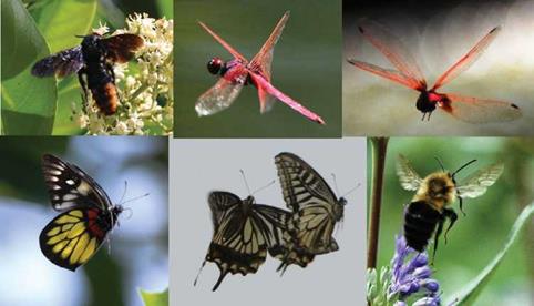
A topic that needs to be addressed more comprehensively is the interaction between fore – and hindwings, and the resulting force and flight control implications. For example, it is well known that dragonflies have the ability to control aerodynamic performance by modulating the phase lag between forewings and hindwings. Wang
|
Figure 5.1. The relative sizes of the insect’s fore – and hindwings are different between species, and consequently, the phase relationship of their wing movement also varies. |
and Russell [533] filmed the wing motion of a tethered dragonfly and computed the aerodynamic force and power as a function of the phase. They found that the out – of-phase motion as seen in steady hovering uses nearly minimal power to generate the required force to balance the weight, and the in-phase motion seen in takeoffs provides an additional force for acceleration. Thomas et al. [258] and Wang and Sun [534] studied the fore- and hindwing interactions via flow visualization and computational simulations, respectively. Brackenbury [535] used high-speed flash photography to analyze wing movements in more than 30 species of butterflies. He observed that early in the upstroke the wings show pronounced ventral flexure that, combined with inertial lag in the posterior parts of both wing pairs and delayed supination in the hindwing, leads to the formation of a funnel-like space between the wings. As shown in Figure 5.1, the relative sizes of fore – and hindwings differ between species, and consequently, the phase relationship of their wing movement also varies. The wing-to-wing interactions are complicated due to a large number of parameters involved. Depending on the flight mission (takeoff, climbing cruising, landing), the fluid physics, such as the leading-edge vortex, wake, and tip vortices; the wing geometry including size, shape, and aspect ratio; and the structural flexibility of the wings all play roles in coupled manners. Wings and body interactions and relative movement are so far largely open research topics.
Much work remains to be done in modeling robust aerodynamics models that can be used to develop control strategies and designs of flapping wing MAVs. As discussed in Chapter 3 most investigations attempting to reduce the complex aerodynamics of flapping wings are fragmented. There is a need for a coherent systematic effort involving simplified analytic theories, high-fidelity numerical simulations, and experimentalists to discern the “quasi-steadiness” of the forces on a flapping wing and to document the validity of these simplified models for various configurations and dimensionless parameters, such as k, St, phase lag, and so on. As already reviewed, Gogulapati and Friedmann [367] offer an updated approach to treat the flapping wing aerodynamics in a simplified framework. Progress is being made in this direction; however, more comprehensive guidelines are needed to establish viscous flow features such as leading-edge vortices and wakes, which depend on these dimensionless parameters. Furthermore, if a wing is flexible, then the viscous and flexible structure interaction becomes significantly more complicated. Gogulap – ati et al. [536] have made an effort in this direction while awaiting the development of a more rigorous approach.
As discussed in Chapter 4, the translational forces resulted from the quasi-steady model for the uncorrected (based on nominal AoA), corrected with the downwash for the flexible, and the rigid wings are highlighted in the figure as well. Clearly, the modifications in (i) effective AoA and (ii) shape deformation affect the aerodynamic performance significantly. The quasi-steady model’s performance can improve noticeably if we know how to correct the effective, instantaneous AoA as well as shape deformation. Without knowing the instantaneous flow field comprehensively, such corrections are difficult to make. More efforts are needed in establishing better guidelines to use such simplified aerodynamic models more effectively.
Regarding the dynamics and stability of a flight vehicle in association with flapping wing aerodynamics, Orlowski and Girard [537] presented a recent overview of various analyses of flight dynamics, stability, and control. Although efforts are being made to use the multi-body flight dynamics model to predict the behavior of flapping wing MAVs, the majority of the flight dynamics research still involves the standard aircraft (6DOF) equations of motion [537]. Furthermore, the investigations of the stability of flapping wing MAVs have so far been essentially limited to hover and steady forward flight, with most studies focusing on linear, time-invariant aspects on the basis of reference flight conditions. Based on such approaches, flapping wing MAVs have been found to be intrinsically unstable in an open loop setting [538]-
[544] . Moreover, control of flapping wing MAVs has been largely investigated by neglecting the mass of the wings on the position and orientation of the central body
[545] -[549]. As summarized in Chapter 1, the ratio between the wing mass and the mass of the vehicle can be of order 0(1), which means that the motion of the wing can affect vehicle dynamics and stability. Natural flyers are often sensor-rich, and these sensors can offer necessary information needed for real-time flight maneuvers in uncertain and unpredictable flight environments. For example, vision-based sensing techniques can be very helpful for flight control as well as for estimating the aeroelastic states of the vehicle.
It is established in Chapter 4 that local flexibility can significantly affect aerodynamics in both fixed and flapping wings. Preliminary research has been reported the vehicle stabilization via passive shape deformation due to flexible structures [550]. Furthermore, as already discussed, insects’ wing properties are anisotropic, with the spanwise bending stiffness about 1 to 2 orders of magnitude larger than the chordwise bending one. As the vehicle size changes, the scaling parameters cannot all maintain invariance due to the different scaling trends associated with them. This means that, for measurement precision, instrumentation preference, and the like, one cannot do laboratory tests of a flapping wing design using different sizes or flapping frequencies [450] [ 551]. A closely coordinated computational and experimental framework is needed to facilitate the exploration of the vast design space (which can have O(102) or more design variables including geometry, material properties, kinematics, flight conditions, and environmental parameters) while searching for optimal and robust designs.
Natural flyers and swimmers share many similarities in terms of the physical mechanisms for locomotion. Although lift is more important for flight than for swimming, pitch, plunge, and flexible structures are all clearly observable in force generation. The difference in density between air and water directly influences the structural properties and some other parameters. However, from a scaling viewpoint, these differences can be linked via the same dimensionless parameters. Much of the same scaling laws are equally applicable to swimming as to flight [37] [38] [41] [186]
[552] [553].
Further, cross-fertilization has been regularly achieved in areas related to locomotion, energetics, morphology, and hydrodynamics. Of course, more interactions are to be expected. For example, Weihs [554] used the slender body theory from aerodynamics to study the turning mechanism in fishes. He showed that the turning process includes three stages, distinguished by different movements of the center of mass. In the first and third stages the center of mass moves in straight lines in the initial and final directions of swimming, whereas in the middle period it moves along an approximately circular connecting arc. The forces and moments acting on the fish can be satisfactorily predicted by treating the vortex wake by the circulation shed from the fins. Weihs [555] also showed that fish can swim more efficiently by alternating periods of accelerated motion and powerless gliding. His analysis of the mechanics of swimming showed that large savings of more than 50 percent in the energy required to traverse a given distance can be obtained by such means. In calculations based on measured data for salmon and haddock, the possibility of range increases of up to three times the range at constant speed was demonstrated. Wu
[553] reviewed the forward swimming motion, bird flight approximated by oscillating wings, and insect flight with the high-lift generation via LEVs. From these studies he derived mechanical and biological principles for unified studies on the energetics in deriving metabolic power for animal locomotion. Studies such as these can offer significant insight into analyzing and designing flapping wing flyers.
Biological and physical scientists and engineers can benefit from close collaboration to better understand features that enable natural flight. For instance, although wings produce lift required for flight in natural systems, not all wing features are flight related. Honeybees employ short-amplitude high-frequency strokes when they hover [556]; these strokes generate high lift as these flyers consume floral nectar containing high energy, which enables them to carry loads or perform high-power-required maneuvers or missions. However, these strokes are shown to be aerodynamically inefficient [216] [351] [404]. Furthermore, bird wings, bat wing membranes, insect wings, and the like have some interesting but widely varied material properties, which can be used for flapping MAV development. These bio-inspired mechanisms include, for example, joints and distributed actuation to enable flapping and morphing. Another topic of much interest but that has so far not been adequately covered is the flight envelope from takeoff to landing. For flapping flyers, key advantages are the variable speed and flapping kinematics along with shape deformation, resulting in highly maneuverable flight characteristics. Furthermore, depending on each species’
|
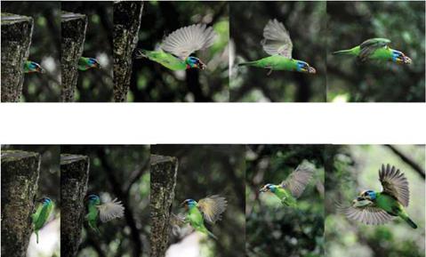
Figure 5.2. The Formosan (Taiwan) Barbet (Megalaima nuchalis), nests in tree cavities, and, as shown in the upper row, forms a noticeably inflated body contour immediately prior to takeoff from the cavity. As shown in the lower row, it also balances delicately between speed and position control to land. |
biological development, its key features in takeoff and landing/perching can vary more than the flapping patterns in comparison to other flyers of comparable sizes. An interesting example is the Formosan (Taiwan) Barbet (Megalaima nuchalis), which nests in tree cavities (see Fig. 5.2). Consequently, they take off with distinctive body movement to generate the initial thrust, including a noticeably inflated body contour immediately prior to take-off. The landing requires a balancing act between speed and position control (see Fig. 5.2.).
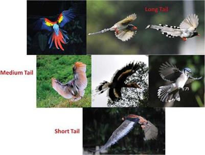
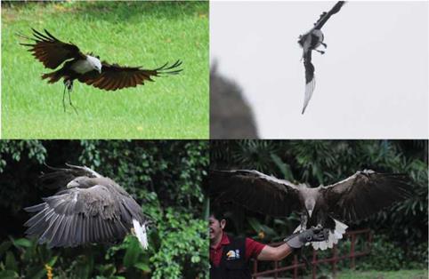
Birds enjoy maneuvering flexibility by combining wings and tails, especially during take-off and landing. However, depending on the individual cases, the relative size of the tail varies significantly. While the parrot and magpie exhibit relatively longer tails than most birds, some birds feature noticeably short tails. These characteristics have major implications on aerodynamics, active and flexible structures, and above all, flight control. Figure 5.3 highlights these features. Another interesting features related to bird flight are that the shape of a wing can be apparently less than streamlined. As shown in Figure 5.4, during takeoff, feather can intrude into the surrounding flows, whose impact is yet to be quantitatively characterized.
Another example is related to hovering. In Chapter 1, it is reported that many birds and bats hover with the stroke plane inclined about 30 degrees to the horizontal, and the resultant downward stroke force with a lift-to-drag ratio of 1.7 is vertical [70]. However, flight environment, especially wind, and vehicle size, can cause strong impact on the hovering pattern. Two small birds, the Ruby-throated Hummingbird (7-9 cm total length) and the Light-vented Bulbul (Pycnonotus sinensis), also known as the Chinese Bulbul (15-20 cm long), can be used as examples here. The flapping of a hummingbird is on a horizontally-inclined stroke plane with a symmetric
|
Figure 5.3. Birds enjoy maneuvering flexibility by combining wings and tails, especially during take-off and landing. However, depending on the individual cases, the relative size of the tail varies significantly. While parrot and magpie exhibit relatively longer tails, some birds feature noticeably shorter tails, resulting in apparently different flight control patterns. |
|
Figure 5.4. During takeoff, feather in certain portion of the bird wing can intrude into the surrounding flow field. |
 |
Figure 5.5. Hummingbirds utilize wing-wail coordination and varied inclination toaccommo – date wind.
figure-eight pattern. Furthermore, as shown in Figure 5.5, due to its small size and light weight, a hummingbird frequently utilizes wing-tail combination and flexible wing structures to accommodate wind gust. Unlike the hummingbird, the bulbul flaps asymmetrically while hovering. As shown in Figure 5.6, in the downward stroke, bulbuls’ horizontally inclined wings move while being rotated. During the upward stroke, the wings are initially flexed and then spread out horizontally. Consequently, lift is generated during the downward stroke; the forward and backward thrusts created during different strokes cancel each other. In short, hummingbirds and bulbuls, both small in size, use distinctively different flapping kinematics, wing morphology and structural flexibility while hovering. Many outstanding issues related to flapping
wing aerodynamics are to be investigated even for commonly observed phenomena. Such complex and varied flight patterns vividly show how much room we have to further learn from nature. By working across the scientific disciplines, scientists and engineers will be able better equipped to uncover the magic of natural flyers’ amazing performance as well as contribute to the advancement of the human-engineered MAVs.

[1] The Passeriform model (herons, falcons, hawks, eagles, and owls): s ~ m078
[2] The Shorebird model (doves, parrots, geese, swans, and albatross): s ~ m071.
[3] The Duck model (grebes, loons, and coots):s ~ m078.
These relations are consistent with those presented in Table 1.3 for all birds other than hummingbirds.
Flexible wings have been found to be beneficial for both natural and human-made flyers. Birds can flex their wings during upstroke to minimize the drag and can still maintain a smooth surface by sliding their feathers over each other. Bats, whose wings consist of membrane and arm bones, can only flex their wings a bit to avoid structure failure or flutter; however, they can enlarge the wing camber during the downstroke. Insects can bend the wing chordwise to generate camber while preventing bending in the spanwise direction.
Fixed, flexible wings can facilitate steadier, better controlled flight. In a gusty environment, a flexible wing can provide a more consistent lift-to-drag ratio than can a rigid wing by adaptively adjusting the camber in accordance with the instantaneous flow field. By responding to the aerodynamic loading variations, a membrane wing can also adaptively conduct passive camber control to delay stall. Moreover, a flexible wing can adjust the wing shape to its motion to mitigate the loss of lift due to the non-linear wing-wake interaction, which can be significant for a rigid wing in hover.
A membrane wing is found to exhibit flutter, whose frequency is about an order of magnitude higher than that of the vortex shedding frequency. The flutter exists even under a steady-state free-stream condition. Such intrinsic vibrations result from coupled aerodynamics and structural dynamics.
We also highlighted the impacts of the anisotropic nature of flexibility on resulting flight performance by considering the chordwise, spanwise, isotropic, and anisotropic wing flexibilities individually. Chordwise and spanwise flexibilities interact with surrounding air, and depending on the imposed kinematics and wing flexibility, they can enhance propulsive force. Studies on anisotropic wing structures are more recent and can provide insightful observations that can be applied to MAV development. The impact of structural flexibility on aerodynamics undergoing plunging motion in forward flight can be highlighted as follows:
1. The thrust generation consists of contributions due to both leading-edge suction
and the pressure projection of the chordwise deformed rear foil. When the rear
foil’s flexibility increases, the thrust of the teardrop element decreases, as does the effective angle of attack.
2. Within a certain range, as chordwise flexibility increases, even though the effective angle of attack and the net aerodynamic force are reduced due to chordwise shape deformation, both mean and instantaneous thrust are enhanced due to the increase in the projected area normal to the flight trajectory.
3. For the spanwise flexible case, correlations of the motion from the root to the tip play a role. Within a suitably selected range of spanwise flexibility, the effective angle of attack and thrust forces of a plunging wing are enhanced due to the wing deformations.
Furthermore, we have demonstrated that as the Reynolds number drops to O(102)- O(103), which corresponds to flyers such as fruit flies and honey bees, the viscous effects are significant, and the flexibility of the wing structure can noticeably change the instantaneous, effective angle of attack via the large-scale vertical flows. The structural flexibility can also mitigate the induced downward jet via shape deformation. Both effects can result in enhanced aerodynamic performance. Furthermore, lift generated on the flexible wing scales with the relative tip deformation parameter, whereas the optimal lift is obtained when the wing deformation synchronizes with the imposed translation, which we also observe in fruit flies and honey bees. Hence, under such modest Reynolds number, the observation that synchronized rotation is aerodynamically preferable for flexible wings is different from what we observe for the rigid wing. It is recalled that in Chapter 3, we have concluded that appropriate combinations of advanced rotation and dynamic stall associated with large AoAs can produce more favorable lift. These findings clearly highlight the effect of wing flexibility.
Since the various scaling parameters vary with the length and time scales in different proportionality, the scaling invariance of both fluid dynamics and structural dynamics as the size changes is fundamentally difficult and challenging. It also seems that there is a desirable level of structural flexibility to support desirable aerodynamics. Significant work needs to be done to better understand the interaction between structural flexibility and aerodynamic performance under unpredictable wind gust conditions. Dimensional analysis and non-dimensionalization of the governing equations for the fluid and the wing structure lead to a system of non-dimensional parameters, such as Reynolds number (Re), reduced frequency (k), Strouhal number (St), aspect ratio (AR), effective stiffness (П1), effective AoA (ae), thickness ratio (h*), the density ratio (p*), and finally the force coefficients. Compared to the set of parameters in rigid flapping wing aerodynamics, three additional non-dimensional parameters were introduced: П1; p*, and h*. From the scaling arguments, the time – averaged force cofficient could be related to non-dimensional relative tip deformation. The tip deformation is an outcome of the interplay between the imposed kinematics and the response of the wing structure dictated by the wingtip amplitude and the phase lag. The amplitude of the maximum relative wingtip deformation, у, was obtained from the non-dimensional beam analysis and is only a function of the a priori known non-dimensional paramters. By considering the energy balance of the wing, the time-averaged force normalized by the effective stiffness was related to y . The time-averaged force can be related to the resultant force on the wing depending on the situation, such as fluid/inertial force, with/without free-stream, or thrust/lift/weight. These results enable us to estimate the order of magnitude of the time-averaged force generation for a flexible flapping wing using a priori known parameters. Furthermore, for propulsive efficiency it was seen that the optimal efficiency was obtained for the motion frequency that is lower than the natural frequency. The current scaling shows that smaller flyers need to flap faster from the efficiency point of view, but the relative payload capacity increases because their weight reduces at a much faster rate compared to larger flyers.
The study of hawkmoth hovering suggests that flexibilty plays a role in both the resulting wing kinematics and aerodynamic force generation. However, because of the limited number of studies regarding fluid-structure interaction in biological flyer-like models, further investigations are needed to derive general conclusions regarding the role of wing flexibility in their flights.

delayed burst of the leading-edge vortex. Aerodynamic and inertial forces applied on a flapping wing can result in passive wing deformations, which are likely responsible for stabilizing and hence delaying the breakdown of the LEV/TiV during wing translation. As illustrated in Figure 4.55c, both flexible and rigid wings show a similar high peak of vertical force immediately after the wing turns to decelerate.
This is because the LEV keeps growing and attaching coherently onto the wing surface, even after the LEV breaks down with the TV shedding off the wing surface [225] [ 388]. However, there exists a pronounced discrepancy at the early downstroke where the flexible wing obviously creates more vertical forces than the rigid wing (Fig. 4.55c). At instance A, a stronger LEV as a portion of a horseshoe vortex is observed near the wingtip of the flexible wing, which grows rapidly over instances of B, C, and D, resulting in a larger and stronger negative pressure region on the wing surface (Fig. 4.55e). Apparently, the spanwise bending of the flexible wing induced during pronation creates this LEV at an earlier timing than in the rigid wing (Fig. 4.56a), which leads to a fast and steep increase in vertical force at A-B (Fig. 4.55c). The LEV then keeps growing for a while up to instance D before approaching the middle down – and upstroke. During the interval, although the inertial force becomes very small (Fig. 4.56i), the spanwise bending and twist and hence the angular velocities show significant variations near the wingtip (B and C; the marked circle in Figure 4.55b). These wing deformations very likely stabilize the LEV and hence result in a delayed burst (breakdown) at D compared with that of the rigid wing at C (Fig. 4.55e). This delayed burst even further influences the development of the LEV after the breakdown, and subsequently the flexible wing reaches a higher force peak than in the rigid wing (Fig. 4.55c). Furthermore, a nose-down twist (Figs. 4.55 and 4.56) can result in a pronounced direction change of the spanwise wing cross-sections, and hence in the direction of force vectors (Fig. 4.55) and the downwashes.
phase advance and angular velocity increases. As seen in Figure 4.55a, the timing of wing twist is adjusted in a passive but adaptive way to advance the phase of wing rotation. This phenomenon is also observed in 2D studies regarding chord – wise flexibility. Moreover, the spanwise flexibility can cause a spanwise bending and hence delays the timing of stroke reversal at the wingtip. Therefore appropriate combination of the chord – and spanwise deformation leads to a relative phase advance of rotation in flexible wings, which can strengthen the vortex ring and the downwash, as well as the rotational circulation, while modifying the wing attitude to benefit from the wake capture [201].
In addition, the wing deformations seem to lead to increasing angular velocities of positional and feathering angles, mostly in the distal area of flapping wings (Fig. 4.55), which can augment the circulation around insect wings [291]. Obviously, the relative phase advance and the angular velocity increase correspond with a larger vertical force (Fig. 4.55), rather than that of the rigid wing during wing rotation. Hence the spanwise bending is responsible for most vertical forces produced immediately before stroke reversal (Fig. 4.55). Furthermore, the rigid wing model with the deformed wing kinematics prescribed (Fig. 4.55) does provide concrete evidence that not only the three-dimensional wing configuration but also the variation in wing kinematics can enhance the aerodynamic force production. In relation to the downwash and the force production, the stronger downward flow (Fig. 4.57) is created in a timely fashion when the wing experiences a rapid stroke reversal where larger forces are created (Fig. 4.55), which was also confirmed experimentally by Mountcastle and Daniel [473].
As noted by Nakata and Liu [523], a rigid wing model with the prescribed wingtip kinematics can create a large vertical aerodynamic force comparable with that of the

 f % t * ** *■ * < < < * * ^
і/ ф Ф ■l Ф downwash generated |Я
7 lYi ^ ^ suPination v v
![]()
vr vv
£ і downwash generated by translation
Non-dimensional downward
flow velocity
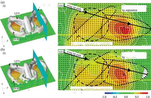
Figure 4.57. Wake structures generated at downstroke about (a) flexible and (b) rigid wings.
(i) Iso-vorticity surface is plotted with a magnitude of 1.5; downwash at a horizontal plane and
(ii) at a cutting plane of 0.6 R from the wing root is visualized in terms of velocity vectors and downward velocity contours. Note that DVR stands for the downstroke vortex ring. From Nakata and Liu [523].
flexible wing; however, this force results in a significant drop in aerodynamic efficiency of 39.8 percent. Furthermore, the efficiency enhancement attained by flexible wings requires more input power. This is because the wing kinematics at the wingtip is modified passively – but favorably – due to the elastic wing deformation, albeit with an input of relatively inefficient wing kinematics at the wing base. Note that the wing base in hovering has low velocity and is ineffective for aerodynamic force production. This suggests that there may be an optimal distribution of wing kinematics between the wing base and wingtip, which should be more efficient in creating vertical aerodynamic forces; see also the discussion in Section 4.5. This points to the importance of the dynamic spanwise distribution of wing kinematics in enhancing aerodynamic efficiency and thus confirms that the elastic wing deformation is an effective way to achieve higher aerodynamic performance in insect flapping flight.
How do these deformations affect the force generation? Time courses of vertical and horizontal force coefficients and aerodynamic force vectors generated by flexible and rigid wings are plotted in Figure 4.55c and d. Although both flexible and rigid wings show a plateau in the vertical aerodynamic force production at early downstroke, the flexible wing obviously creates more force than the rigid wing, and the force vectors contribute more to the vertical force components (Fig. 4.55c, d). Instantaneous
streamlines and pressure contours on the wing surfaces are illustrated in Figure 4.55e during an interval where four instants are marked as A, B, C, and D (Fig. 4.55e). At early downstroke when the wing proceeds to late pronation and undergoes a pitch-down rotation, the LEV and the TEV grow in size and in strength, stretching from the wing base toward the wingtip; the TEV subsequently detaches from the wing, forming a starting vortex but connecting to the LEV and the TiV at the wingtip at A (Fig. 4.55e). Subsequently, the TiV of the rigid wing becomes unstable at C, gradually separating and shedding from the wing surface, which correspondingly results in a shrink pattern of low-pressure contours at the wingtip. In contrast, the LEV and the TiV on the flexible wing seem to be more stable than those of the rigid wing, with an enlarged low-pressure region at B and C (Fig. 4.55e). When the TiV
|
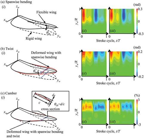
Figure 4.56. (i): Definition of the simulated (a) spanwise bending angle, (b) twist angle, and (c) camber in the flexible wing. (ii) Time courses and spanwise distribution of the three kinds of deformation of a flexible wing and (iii) their interpolated deformation. From Nakata and Liu [523]. |
breaks down and separates from the wing, the LEV still keeps growing with a strong low-pressure region at D (Fig. 4.55e) until the vertical aerodynamic forces generated by both flexible and rigid wings become almost even immediately after the wing turns to decelerate. However, it is interesting to find that, at late downstroke, the flexible wing eventually reaches a higher force peak other than the rigid wing (Fig. 4.55c). When the wing approaches early supination, the aerodynamic force decreases owing to the breakdown or shedding of the LEV and the translational deceleration. Here, the flexible wing can also create larger forces than the rigid wing.
As discussed earlier, there are few studies of the aerodynamics of flapping wings associated with anisotropic wing structure; in addition, the 3D wing shape and the timing of deformation during flapping flight have not yet been studied well. Recently, Nakata and Liu [523] conducted a computational analysis of hawkmoth hovering flight based on a realistic wing-body model, which takes into account the anisotropy of a hawkmoth wing. They investigated how the wing deformation and modified kinematics due to the inherent structural flexibility affect unsteady fluid physics and aerodynamic performance. In their study, a reasonably representative wing – body morphological model was built as shown in Figure 4.54. Note that although hawkmoths are four-winged, for simplicity, they modeled the fore – and hindwings as a single pair of wings because of the highly synchronized motion observed in flapping flight. Hawkmoths’ wing structure is mainly supported by wing veins and membrane. The wing veins are clustered and thickened around the wing base and leading edge, as illustrated in Figure 4.54a, and are tapered toward the wingtip and trailing edge [403] [524]. A thin flexible membrane is placed between the veins; the directional arrangement of the wing veins and the difference of bending stiffness between the veins and membrane result in a high anisotropy of the flexural stiffness of hawkmoth wings [402]. Wing and body kinematic models were constructed based
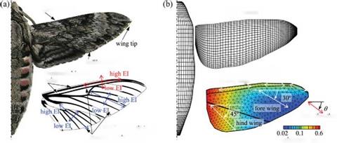 El: flexural stiffness

structural anisotropy
Figure 4.54. (a): A hawkmoth Agrius Convolvuli with a generalized wing venation including fore – and hind-wings. (b) A computational model for CFD and CSD analysis. From Nakata and Liu [523].
on the experimental data of the hovering hawkmoth, Manduca, and on kinematic parameters [247] [523] described in Section 3.7. Note that the body was assumed to be stationary because the body motion in hovering flight is negligibly small [226].
2.6.1.1 In-Flight Deformation of a Hawkmoth’s Wing
Figure 4.55 shows the comparison of the instantaneous and time-averaged results associated with flexible and rigid wings. Figure 4.56 displays the time-varying wing shape and deformation in terms of the spanwise bending, the twist, and the camber. From Figure 4.55a the flexible wing shows an advanced phase in the feathering angle, but a delayed phase in the positional angle at the wingtip, with respect to prescribed motion of the rigid wing at the wingtip. Also from Figure 4.55b, the translational and rotational velocities in the cross-section of 0.8R increase remarkably, in particular before stroke reversal. Those results occur because of large spanwise bending and twisting when the wing translates and because of small peaks before the subsequent stroke reversal as illustrated in Figure 4.56. Furthermore, although the spanwise bending and the twist angle vary smoothly, there exists a rapid increase in distal area. The flexible wings show pronounced deformation in spanwise bending and twist immediately after stroke reversal. The maximum of nose-down twist in the distal area (forewing) is approximately 12° when predicted by computation and 15° ~ 20° when measured by experimentally [226]. One can see some positive camber, less than 2 percent, that is relatively small compared with the measured cambers of large insects such as locusts [525]. Overall, such deformation leads to significant changes in wingtip kinematics.
Recently, efforts have been made to directly investigate the aerodynamic performance of biological flyers while accounting for the effect of flexible wing structures.
For example, Agrawal and Agrawal [518] investigated the benefits of insect wing flexibility on flapping wing aerodynamics based on experiments and numerical simulations at Re of 7.0 x 10³. They compared the performance of two synthetic wings: (i) a flexible wing based on a bio-inspired design of the hawkmoth wing and (ii) a rigid wing of similar geometry. The results demonstrated that the bio-inspired flexible wing generated more thrust than the rigid wing in all wing kinematic patterns considered. They emphasized that the results provided motivation for exploring the advantages of passive deformation through wing flexibility.
Singh and Chopra [519] experimentally measured the thrust generated for a number of wing designs undergoing flapping motion at Re of 1.5 x 10⁴. The key conclusions that stemmed from this study were that the inertial loads constitute the major portion of the total loads acting on the flapping wings tested on the mechanism and that, for all the wings tested, the thrust drops at higher frequencies. Further, it was observed that at such frequencies, the lightweight and highly flexible wings used in the study exhibit significant aeroelastic effects.
Hamamoto et al. [520] studied FSI analysis on a deformable dragonfly-like wing in hover and examined the advantages and disadvantages of flexibility at an Re of 1.0 x 10³. They tested three types of flapping flight: a flexible wing driven by dragonfly flapping motion, a rigid wing (stiffened version of the original flexible dragonfly wing) driven by dragonfly flapping motion, and a rigid wing driven by modified flapping based on tip motion of the flexible wing. They found that the flexible wing with nearly the same average energy consumption generates almost the same amount of lift force as the rigid wing with modified flapping motion. In this case, the motion of the tip of the flexible wing provides equivalent lift to that provided by the motion of the root of the rigid wing. However, the rigid wing requires 19 percent more peak torque and 34 percent more peak power, indicating the usefulness of wing flexibility.
Young et al. [521] conducted numerical investigations on a tethered desert locust, Schistocerca gregaria. Their results showed that time-varying wing twist and camber are essential for the maintenance of the attached flow at the Reynolds number, 4 x 10³. The authors emphasized that, although high-lift aerodynamics are typically associated with massive flow separation and large LEVs, when high lift is not required, attached flow aerodynamics can offer greater efficiency. Their results further showed that, in designing robust lightweight wings that can support efficient attached flow, it is important to build wings that undergo appropriate aeroelastic wing deformation through the course of a wing beat.
Tanaka et al. [522] investigated the effect of wing flexibility in hoverflies using an at-scale mechanical model. They suggested that at-scale models operating in air have the potential to simulate the aerodynamic phenomena of compliant flapping wings because their structure, inertia, operating frequency, and trajectories are similar to those of insects in free flight. For this purpose, an at-scale polymer wing mimicking a hoverfly was fabricated using a custom micro-molding process. It had venation and corrugation profiles that mimic those of a hoverfly wing, and its measured flexural stiffness was comparable to that of the natural wing. To emulate the torsional flexibility at the wing-body joint, a discrete flexure hinge was created. A range of flexure stiffness was chosen to match the torsional stiffness of pronation and supination in a hoverfly wing. The polymer wing was compared with a rigid, flat,
![]()
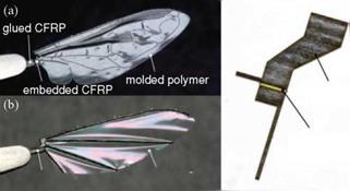 Polyester film
Figure 4.53. Photos of an at-scaled model wing: (a) hoverfly mimic; (b) a rigid carbon fiber model; and (c) example of hinge. The wing length is 11.7 x 10³ [m]. From Tanaka et al. [522].
carbon-fiber wing using a flapping mechanism driven by a piezoelectric actuator as shown in Figure 4.53. Both wings exhibited passive rotation around the wing hinge; however, these rotations were reduced in the case of the compliant polymer wing due to chordwise deformations during flapping that caused a reduced effective AoA. Maximum lift was achieved when the stiffness of the hinges was similar to that of a hoverfly in both wing cases and the magnitude of measured lift was sufficient for hovering. These results suggest that hoverflies could exploit intrinsic compliances to generate desired motions of the wing and that, for the same flapping motions, a rigid wing could be more suitable for producing large lift.
In the next several subsections, we summarize recently reported studies based on biological models.
The time-averaged force (CF) and the propulsive efficiency n could be related to the resultant force on the wing depending on the situation, such as fluid/inertial force, with/without free-stream, or thrust/lift/weight. The current result enables us to estimate the order of magnitude of the time-averaged force generation and and its efficiency for a flexible flapping wing using a priori known parameters.
Furthermore, the scaling can guide the design of flapping wing MAVs. For example, to support a given weight Wbody of a vehicle body in air, the scaling Eq. (4-36) reduces to
![]()
![]()
p 1r3.19 f2.38ф2.19с1.57 ps фа m
h038E019
m0.42g0.42h0.16 e0080
p0.42 о1.34ф0.92с0.66 ps фа m
assuming П1 > П0. The condition П1 > П0 is satisfied when f1 > f and simplifies the algebra; however, it poses constraints on the range of the structural properties, such that the natural frequency of the wing is higher than the motion frequency. Equation (4-48) shows that increasing either the wing area, motion frequency, or the flapping amplitude helps generate sufficient lift to sustain hovering flight. In contrast, by making the wing softer (i. e., reducing the Young’s modulus or wing thickness), wing deformations will increase, leading to higher lift generation. However, softening the wing further will violate the frequency ratio assumption, f1/ f > 1. The relation given for the flapping frequency is similar to that identified by Pennycuick [59]. Note that the wing weight is assumed to be negligible compared to the body weight in Eq. (4-48).
Another implication of the scaling is the interesting behavior of the role of h* for the chordwise flexible airfoil cases shown in Section 4.3.2. It was observed that the CtI increased first and then decreased with decreasing h*; see Figure 4.31. Using the current scaling, which is repeated as
1.17
consider first the situation that f1 > f, i. e., h* is not small. Then the denominator in
|
( |
k4 П I
4J5П – і ^ Пі, yielding
hence by reducing the thickness ratio, Пі ~ hf will decrease, leading to the observed enhanced [Ct). However, by decreasing h* further, the frequency ratio f1/f will be eventually of the same order of magnitude, resulting in different physical behavior. If, say f1/f = 0(1), but not in the resonance region, then the denominator in у will scale as П0 j 4^ П ^ « П0. Then, the resulting scaling will be
 |
 |
Figure 4.52. Force and propulsive efficiency plotted against the frequency ratio f/f1.
Sincen1 ~ hf and П0 ~ h,*, we have Ct) ~ h)183. This is consistent with the trend shown in Figure 4.31 that reducing the thickness ratio further will reduce the thrust.
Furthermore, for the thrust scaling for flapping flexible wings in water in forward motion, Eq. (4-37) can be rewritten as
1.17
and since St ~ ю, к ~ ю, and П0 ~ к2 ~ ю2, the thrust has a maximum at the resonance frequency. In reality, there is damping in the system, either structural or aerodynamic [456]. Although the effects of damping are not considered here, applying those effects for linear oscillators (e. g., [515]) yields the resonance frequency slightly below the natural frequency of the wing, with a finite value for the maximum relative wingtip deformation and hence the thrust: see Figure 4.52. In Figure 4.52b the effects of damping have been incorporated by approximating the denominator term as
|
Table 4.4. Optimal frequency ratios reported in the literature
|
where d is some small damping coefficient. This finding is consistent with the previous findings that the optimal propulsive performance is found near but slightly below the natural frequency of the wing [222] [453] [454] [508].
The propulsive efficiency scaling Eq. (4-47) can be rewritten in terms of the frequency ratio f/f1 as
|
|
which has a local maximum at f = 0.41f1. Depending on the scaling of the force, the optimal frequency can be found as
dj = 0 ^ f lopt =Ув-ї, (4-55)
where в is the exponent of у in the force scaling (i. e., 1.17 in Eq. (4-37) or 1.19 in Eq. (4-47), which yields the optimal frequency of 0.41 of the natural frequency. This indicates that the optimal efficiency is not achieved at the resonance frequency, but that the optimal frequency is some fraction of the natural frequency of the wing, which is also consistent with previous findings in the literature [453] [454] [492] [510] [516]; see Table 4.4. A cautionary note should be made, however, that Eq. (4-52) is derived from Eq. (4-36) and assumes f / f1 < 1. Hence, strictly speaking, the conclusion that the maximum force is generated at the resonance frequency is not valid. The revised scaling proposed by Kang and Shyy [404] by considering hovering flexible flat plates cases with frequency ratios up to 0.8 would yield the frequency ratio of 0.6 without including the effects of damping.
Figure 4.52c depicts Eq. (4-55) as a function of the frequency ratio and shows that the propulsive efficiency increases with the increasing frequency ratio until reaching the optimal efficiency, and then it drops to zero at the resonance frequency. Since the undamped linear oscillator is unable to represent the resonance behavior correctly, an arbitrary damping has to be included in the system as before. Figure 4.52b shows the effects of including damping, where d is taken to be 0.0,0.2, and 0.4: the optimal frequency ratio increases with increasing d, as does the efficiency at the resonance frequency. Note also the similarity between Figure 4.52b and the computed propulsive efficiency curves shown in Figure 4.48. A qualitative comparison with the measurements reported in Ramananarivo, Godoy-Diana, and Thiria [454] shows that, although the precise details differ, the overall qualitative trend is similar.
For example, for a 2 percent thickness wing with a rectangular planform made of aluminum hovering in air, the optimal frequency of the flapping motion is 5.4 Hz
Table 4.5. Summary of the proposed scaling
![]()
![Подпись: Force 119 Efficiency в3у117 Source: [351].](/img/3131/image520_2.gif) |
|||||||
Forward locomotion, water
when the wing has a chord length of 20 cm and span of 50 cm with a flapping amplitude of 30°. Scaling down the geometry of the wing 10 times to the chord length of 2 cm and span of 5 cm, and keeping the aspect ratio the same, the optimal flapping frequency increases to 54 Hz. The resulting propulsive force coefficient and the propulsive efficiency remain the same for both cases. However, the dimensional propulsive force and the power required are 100 times smaller for the smaller sized wing, proportional to the square of the chord. Yet, for the same aspect ratio and thickness ratio, the volume of the wing is proportional to the cubic power of the chord. Consequently, for the same material, the mass of the smaller wing is 1,000 times smaller. The current scaling shows, consistent with Shyy et al. [245], that smaller flyers need to flap faster from the efficiency point of view, but their relative payload capacity increases because their weight reduces at a much faster rate compared to larger flyers.
Finally, the scaling parameters for diverse flow and kinematics conditions are summarized in Table 4.5. For forward flight in water, the effective stiffness Пх, the normalized plunge amplitude h*a, the mass ratio p. s = pha/(pshs), and the frequency ratio f/f1 dictate the propulsive force and the efficiency. For hovering in air, for the studied kinematics, the role of the mass ratio is taken over by the factor p*h*a = p, s/h* . Determining the efficiency for the hovering motion in air is left to future work in this study, and the resulting scaling is only predicted by following the same argument as for the propulsive efficiency in forward flight in air. Notice that the factor p*h*a = pha/(pscm) is much smaller than ps = pha/(pshs), resulting in a much lower propulsion for the hovering symmetric flap/plunge motion in air, since the thickness ratio is usually only of the order of 0.01. This order estimation matches well with the values shown in Ramananarivo, Godoy-Diana, and Thiria [454]. For the hovering Zimmerman wing the ratio between the propulsive force CL and the force required for input power, CT, was of the order of h*. This scaling suggests that insects may require different mechanisms, such as active or passive pitching motion with a reinforced leading edge, which is commonly observed in many insect wings (see Fig. 4.4). Furthermore, non-symmetric motions, such as figure-of-eight motion (see Fig. 1.11) where the wing experiences forward motion, may yield higher efficiency [517].
To illustrate the implications of flexible wing further, Kang and Shyy [404] argued that the effects of wing flexibility can be explored from two angles: (i), one can study the equilibrium shape compliance in accordance with the stress distributions around the body. The resulting modification of the angle-of-attack and the wing shape can potentially better adapt, reducing tendencies toward, e. g., massive flow separation and stall. (2), structural dynamics during transient process can offer further time – dependent behavior other than static shape compliance. The interplay of the fluid flow with the shape compliance and transient response is nonlinear and intriguing [557] even at low Reynolds numbers relevant to insect flyers, i. e. Re = O(102).
To isolate these sources of aerodynamic force modification, Kang and Shyy [404] considered a flexible plunging wing operated in translational motion only by prescribing a sinusoidal displacement on the leading-edge (LE) of the wing (Fig. 4.43a). Consequently, the resulting wing camber deformations and rotation a, the angle between the trailing-edge (TE) and LE, are purely passive due to dynamic balance between the aerodynamic loading, elastic restoring force, and inertia of the wing. In order to elicit the effects of flexibility with minimum complexity and ambiguity, a was approximated with a first-order harmonic (FH) approximation using am and ae, the angles at the end and mid-of-the-strokes, respectively, as aFH = 90 – aacos (2nt* + y) by calculating the angular amplitude aa and phase lag ф. Specifically they imposed a and aFH on a rigid flat plate without camber. To elucidate the interplay between the fluid physics and shape compliance they first considered the flexible wing and the rigid wing with a. As shown in Section 4.5.2, the cycle averaged lift coefficients CL versus y covers a wide variety of wing flexibility and flapping characteristics relevant to insects as well as artificially-devised flexible wings (Fig. 4.43b). Parameter y can be interpreted as the non-dimensional wing tip displacement relative to the LE. The chordwise wing deformations act as passive pitch with an angle-of-attack, which is a key measure of the aerodynamics and directly affects lift (Fig. 4.43c).
Additional forces arise at the stroke reversals for rigid wings. When actively rotating wings exert force on the surrounding fluid, the fluid adds to or subtracts from the lift due to delayed stall, or translational mechanisms as described in Section 3.3. Their benefits depend on the phase difference between translation and rotation, advanced rotation being the optimal. Flexible wings also depict these three phase modes via passive rotation (Fig. 4.43d). The phase lag ф strongly correlates to f/f1, yielding the advanced, symmetric, and delayed rotation modes with increasing f/f1 (Fig. 4.43e). However, the large pressure differentials that exist on actively rotating rigid wings near the TE due to lift enhancing rotational effects are relaxed
by the compliant nature of flexible wing. Instead of generating rotational forces, the wing streamlines its shape, such that the wing shape and motion are in equilibrium with the fluid forces, similar to the drag-reducing reconfiguration of flexible bodies. Passive rotational angle a is purely due to deformation where the amplitude and the phase scale with y and f/fx. Moreover, am is measured at the instant of maximum translational velocity, hence indicative of the forces related to the translational mechanisms. For advanced rotations (f/fx < 0.25), am is greater than 70 deg. The
 |
Figure 4.44. Difference in lift between flexible and rigid wings. (a) CL on the flexible and rigid wings as a function of y (b) RMS difference in the lift as a function of log10Y/k2. Time histories of lift for the cases and schematics of wing shapes with the largest and smallest differences in lift are shown in (c, d) and (e, f), respectively. Both cases exhibit symmetric rotations with (c) a high reduced frequency and with (e) a low reduced frequency for the flexible (red), rigid (blue) wings and their instantaneous wing shapes (d, f). From Kang and Shyy [404].
wing orientation is almost vertical, producing small lift. On the other hand, deformations can become substantial for delayed rotations modes with f/f1 > 0.4, but since the translation is out-of-phase with the passive rotation, the resulting am and hence the lift remain smaller than for symmetric rotations. The translational forces peak when am is around 45 to 50 deg, which corresponds to 0.25< f/f1 < 0.4 (Fig. 4.43e). The resulting lift is of similar magnitude to that of rigid wings with active rotations. However, the lift is now optimal for symmetric rotation modes (Fig. 4.43f). This is also observed in the wing kinematics of fruit flies and honeybees.
To further assess the effects of flexibility, Kang and Shyy [404] compared the lift generation on the flexible wing and the rigid wing rotating with аш. Both wings generate lift that scales with y (Fig. 4.44a). Most flexible wings yield higher lift with
 |
|
a difference that depends on y/k2 (Fig. 2B). As у increases, wing deformations become larger and will eventually cause the observed differences. The dependence on k2 can be explained by considering the relative contribution of the added mass force and the forces induced by the vorticity in the flow field as explained in Section 3.6.4, which scale as k and 1/k, respectively, for hover.
As such, at higher k the added mass force, which is linearly proportional to the wing acceleration, has a larger contribution to lift. The impact of the added mass on the total aerodynamic force for both wings remains similar, because the essence of the wing motions is consistent between flexible and rigid wings. Consequently, the resulting lift is close as Figure 4.44c and d.
When the reduced frequency is lowered, aerodynamic force induced by vorticity in the flow field, such as translational forces and nonlinear wing-wake interactions, starts to dominate the lift. These non-linearities in the unsteady aerodynamics lead to intriguing consequences caused by small differences in the resulting non-linear wing motion and the camber deformation. For example, Figure 4.44e illustrates the case corresponding to the largest difference in the lift. Lift on the flexible wing is considerably higher during the midstroke compared to that of the rigid wing (Fig. 4.44e, f), such that the lift generated by the flexible wing is superior: 1.2 versus 0.88.
The simple representation aFH in the study of flapping wings is a popular approximation for rigid wings as shown in Section 3.4.1, despite the observations of hovering fruit flies and honeybees that are clearly far from sinusoidal [228]. Similar to these insects, the resulting flexible wing motion significantly deviates from being a sinusoid, depending on the wing properties (Fig. 4.45a). In general, the lift is higher for rigid wings with a. The dynamic balance between the fluid and the wing structure results in a rotation with larger deformation indicated by amax = max(a) near the midstroke (Fig. 4.45b). The rigid wing following a generates higher lift that correlates to the difference between amax and amax, FH, the angular amplitude in the simple harmonic motion, as illustrated in Figure 4.45c for the most cases. Inversely, this means that better performance can be obtained by departing from a simple sinusoidal rotational motion.
vertical velocity 1.5
![]()
![]()

![]() 0.9
0.9
0.3
-0.3
-0.9
 |
 |
-1.5
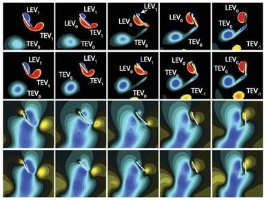
Figure 4.46. Effects of streamlining for a symmetric rotation mode by comparing to the rigid wing rotating with а. (a) Vorticity and vertical velocity fields. The wing thickness is exaggerated for clarity. (b) Schematic illustration of the wing-wake interaction. (c) Time history of lift normalized by c or c(t*) (8). (d) CL as a function of y. (e) Time histories of the vorticity of TEV0 and LEV1 and downwash. From Kang and Shyy [404].
An important mechanism responsible for lift enhancement of flexible wing over its rigid counterpart is due to wing-wake interactions, as highlighted in Figure 4.46. Kang and Shyy [404] considered a flexible and its rigid counterpart, rotating with а to focus solely on the effects of camber deformations. The LEV and the TEV shed in the previous motion stroke, denoted as LEV0 and TEV0, respectively, form a
vortex pair and induce a downward wake around the midstroke, see also Chapter 3, which in turn interacts with the wing during its return stroke. The outcome of the rigid wing-wake interactions varies. Under favorable conditions, added momentum causes the lift to increase during the first portion of the stroke. The wing then experiences two peaks in lift: the wake-capture and the delayed stall peaks as shown in Figure 4.46b. However, the wake can also form a downward flow, causing the lift to drop significantly during midstroke.
A flexible wing, on the other hand, can reconfigure its shape, adjusting its camber to better streamline with the surrounding flow [404]. Consequently, the formation of the TEVs reduces for the flexible wing and the negative impact of the induced downwash is mitigated (Fig. 4.46a, b), leading to higher lift during the midstroke. For a locust, positive camber was measured in the hind wing due to the compression of the veins via trailing-edge tension [224]. The positive camber led to the umbrella effect, enhancing lift in the downstroke [224, 521]. Compared to the locust, whose Reynolds number is Re & 4 x 10³ [224], Figure 4.46 focuses on Re = 100 and different detailed wing characteristics. These lead to different observations: The negative camber has in general less favorable aerodynamic performance. However, for flapping flexible bodies, the streamlining mechanism causes utilization of the translational lift with higher efficiency, while at stroke reversals, it lessens rotation related force enhancement. As a result the time history lift changes from the two – peak shape to one-peak in the middle of the stroke (Fig. 4.46c). The lift enhancement increases with increasing deformations, characterized by y (Fig. 4.46d).
To quantify this streamlining process, Kang and Shyy [404] first measured the vorticity at the point of the highest second invariant of the velocity gradient tensor Q in the TEV0. The vorticity magnitude of TEV0 for the rigid wing is higher, which correlates to a stronger downwash (Fig. 4.46c). They estimated the strength of the downwash by averaging the vertical velocity over a tracking window placed upstream of the wing. Figure 4.46e confirms the stronger downwash depicted in Figure 4.46a for the rigid wing.
The angle-of-attack is a key measure of the aerodynamics, and can directly affect features such as LEV and lift. Since the flow field surrounding a hovering wing is complicated, one needs to define an effective angle-of-attack in order to better characterize the aerodynamics, which Kang and Shyy [404] modeled as a combination of the translational velocity of the wing and the downwash of the surrounding fluid. Furthermore, to estimate the effects of the downwash on the lift, they used the effective angle-of-attack for the translational force term of the quasi-steady model (Fig. 4.47a). The correlation of the resulting quasi-steady lift to the Navier-Stokes solutions substantially improves compared to the estimation without the correction for the downwash (Fig. 4.47b, c). The enhanced agreement suggests that the drop in lift during the midstroke is indeed caused by the wing-wake interaction for the rigid wing (Fig. 4.47c). The flexible wing alleviates the downwash by streamlining its wing shape and outperforms its rigid counterpart with a difference in lift coefficient up to 0.3. The shape compliance and the dynamic responses of the flexible structure together contribute to the lift enhancement. However, without knowing the shape of a deformed flexible wing, the quasi-steady model cannot satisfactorily predict the aerodynamic force. Moreover, its performance can improve noticeably if we know
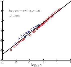
resulting power. The fact that the power required is non-zero means that the resulting instantaneous lift on the wing should have a phase lag relative to the imposed motion. A major source for the phase lag is the wing deformation. By acknowledging the wing deformation given in Eq. (4-34), the time-averaged power input coefficient due to added mass can be approximated as in the first mode:
1
For П1 > П0 the scaling for (CP) reduces to St2{1 + 4p*h*/n); hence (CP) ~ St2 in water, such as in the experimental setup considered in this case [336] [502], or for fixed density ratios and thickness ratios of the wing, consistent with the previous literature [456] [502] and Figure 4.49. Because the scales of (C^ vary enormously, (CP) /в2 is plotted against y in log-scale in Figure 4.50. A linear fit with R2 = 0.98
![]()
From the results presented in Sections 4.4.2.1-4.4.2.3 for the three different cases Kang et al. [351] made the following observations: (i) the time-averaged force increases with increasing motion frequency; (ii) changes in structural properties, such as the thickness ratio, Young’s modulus, or wing density (mass), lead to a non-monotonic response in the force generation; and (iii) for the hovering isotropic Zimmerman wing, the ratio between the density ratio and the effective stiffness is monotonic with the time-averaged lift generation. To explain the observed trends Kang et al. [351] mainly analyzed the physics based on Eq. (4-1) with simplifying approximations for the fluid dynamic force, f*xt (see also Section 3.6.4), based on scaling arguments. The flow field and the structural displacement field should simultaneously satisfy Eq. (3-18) and Eq. (4-1); of these two equations Eq. (4-1) was considered, which has the advantage that it is linear, except for the fluid dynamic force term; in contrast, the Navier-Stokes equation is non-linear in the convection term. Subsequently, a relation between the time-averaged force and the maximum relative tip displacement was established by considering the energy balance.
To capture the essence of the mechanism involved in the force enhancement due to flexibility, it is necessary to analyze the interplay among the imposed kinematics, the structural response of the wing, and the fluid force acting on the wing. The derivation leading to the relation between the time-averaged force acting perpendicular to the wing motion, (Cp) and the maximum relative tip deformation vmax is lengthy, where v* (x*, t*) = w* (x*, t*) – h(t*) is the displacement of the wing relative to the imposed kinematics motion; see Kang et al. [351] for the detailed steps. A treatment using simplifying approximations is helpful in enabling the analysis, but mainly serves to elucidate the scaling analysis and is not meant to offer a complete solution. Consider Eq. (4-26) in one dimension in space with 0 < x* < 1 and time
t* > 0, for the vertical displacement w*, with the wing approximated as a linear beam. A plunge motion, Eq. (3-12), is imposed at the leading edge at x* = 0. The trailing edge x* = 1 is considered as a free end (i. e., with the boundary conditions,
w* (0, t *) = h(t *) = St cos(2n t *), к
and the initial conditions
*, * п дw*(x*, 0)
w* (x, 0) = St, = 0,
( ’ ) к, дt *
where the factors involving l/cm become unity for the chordwise flexible airfoil case). For the spanwise flexible wing and the isotropic Zimmerman wing cases that are discussed in Section 4.4.2.2 and Section 4.4.2.3, respectively, П0 and П need to be corrected as l/cm = AR. Following the procedure described in Mindlin and Goodman [511], a partial differential equation with homogeneous boundary conditions can be found by superimposing the plunge motion on the displacement v(x*, t*) = w(x*, t*) – h(t*). The consequence of having a sinusoidal displacement at the root is that the vibrational response of the wing is equivalent to a sinusoidal excitation force, which is the inertial force. The dynamic motion given by Eq. (3-12) is coupled to the fluid motion via the fluid force term f*xt, which cannot be solved in a closed form due to its non-linearities.
For high-density-ratio FSI systems, Daniel and Combes [470] and Combes and Daniel [472] showed that the inertial force arising from the wing motion is larger than the fluid dynamic forces. To cover a wider range of density ratios, Kang et al. [351] included the fluid dynamic forces by considering the added mass effects. The motivation stems from the scaling discussed in Section 3.6.4, where for high к the added mass terms due to an accelerating body (see also Combes and Daniel [472]) contribute more on the wing than do the fluid dynamic forces from the hydrodynamic impulse; see Table 4.2 for a summary of the non-dimensional numbers considered in this study. Figure 3.55 illustrates the domain of importance of the various effects of the unsteady fluid force. Hence, the wing dynamics is modeled with external forces depending on the imposed wing acceleration as
![]() f*xt (t*) ^ 2п2St к cos(2nt*),
f*xt (t*) ^ 2п2St к cos(2nt*),
and the external force on the structural dynamics does not have spatial distribution explicitly accounted for and is being simplified in temporal form.
When dombined with the inertial force, the total external force g(t*) becomes
g(t*) = f*xt (t*) – П0 d h(l ) « 2п2 1 + — p*h* St к cos(2nt*). (4-31)
dt *2 п
The solution for the tip displacement is given by Kang et al. [351] who used the method of separation; that is, v* (x*, t*) = X(x*)T(t*) as
for the temporal component, with Qn, the Fourier coefficient of a unit function in the spatial modes, satisfying
![]() j XndX Xndx
j XndX Xndx
0
and the natural frequency
with kn as the eigenvalue belonging to the spatial mode Xn with k1L & 1.875. The spatial component Xn is the same as for a cantilevered oscillating beam. The temporal evolution of the wing given by Eq. (4-32) indicates there is an amplification factor of 1 /(f2/ f2 – 1), depending on the ratio between the natural frequency fn of the beam and the excitation frequency f.
The full solution is w*(x*, t*) = h(t*) + J2 n==1Xn (x*)Tn (t*). The amplitude of the tip deformation, у, for the first mode (n = 1) is given as
![]() (1 + Пp*h* ■ st ■ k
(1 + Пp*h* ■ st ■ k
По (f2/ f2 – 1)
relative to the imposed rigid body motion normalized by the chord. The parameter Y can be rewritten as
![]() Y ( P^m ^ + Л 4_________ A + 1
Y ( P^m ^ + Л 4_________ A + 1
ha/cm pshs 4 f^2 – 1 – 1
where f1/ f = ш1 /(2n) is the inverse frequency ratio and A = npcm/(4pshs) is the ratio between the acceleration-reaction force (added mass) and the wing inertia. Depending on the order of this ratio, either the acceleration-reaction force term or the wing inertia force can be neglected. Equation (4-35) gives the relative wingtip deformation normalized by the plunge amplitude, which can be related to the Strouhal number based on the deformed tip displacement. Note that when A is sufficiently large, the inertia force term can be neglected and Y is then proportional to Ah* – pha/(pshs).
The proposed scaling parameter to estimate the resulting force on the flapping wing follows from the observation that there exists a correlation between the dynamic deformation of the wing at the tip, y , given by Eq. (4-34), and the static tip deflection, which is (CF) /Пг. By considering the non-dimensional energy equation, Kang et al. [351] derived the following relation between the time-averaged force [CfI and the maximum relative tip displacement represented with the scaling factor y, under the assumption of f1 / f < 1, resulting in
<Пг> – Y. (4-36)
П1
The resulting scaling – Eq. (4-36) for the three canonical cases – is shown in Figure 4.40. When plotted in the log-scale, see Figure 4.40, the scaling for all cases
considered becomes more evident. A linear fit on the data set with the coefficient of determination of R2 = 0.98 indicates that the relation between the normalized force and y is a power law with the exponent of 1.19. The relation originating from the dimensional analysis, Eq. (4-36), then simplifies to
[CF) = Ui^(y), (4-37)
with ^(y) = 10098y 119. The elastoinertial number, Nei proposed by Thiria and Godoy-Diana [454] as the thrust scaling parameter in air is a special case of y ; that is,
![]()
 |
р*й;»1 and ///1»1
Y——————- ► Nei-
It is important to note that the у-axis in Figure 4.40 shows [CF). Recall that [CF) was defined as the force acting normal to the wing that is responsible for the wing deformation; hence [CF) is normal to [CT) or (CL) depending on the direction of the wing deformation. For the purely plunging chordwise flexible airfoil cases in forward flight in water, [CF) = [CT)/(St ■ k) where the factor St ■ к is the ratio between CL max/ [CT) ~ St ■ к for the added mass force and [CT] by Garrick [335] for purely plunging airfoils. For all chordwise flexible airfoil cases parametrized by (f, h*), (CF) /П1 shows almost a linear correlation with y. Recall that the inertial force term arising from the plunging boundary condition is small compared to the added mass term because for the plunging chordwise flexible airfoils p*h* < 1. Compared to the higher motion frequency cases, the thrust generation at the lowest frequency at the five thicknesses has a larger variance, which is not shown in Figure 4.40. A plausible explanation is that the current analysis breaks down due to the presence of the rigid teardrop at lower motion frequencies. When the plunging
motion is very slow at the rigid teardrop, the large leading-edge radius produces time-averaged drag that overwhelms the thrust generation from the thin flat plate with small deflection. The airfoil produces drag at St = 0.085 on all five thickness ratios as shown in Figure 4.40, which would result in an under-predicted value of
CL /П1.
For the spanwise flexible wing, although the Reynolds number and the thrust direction relative to the wing flexibility are different than in the chordwise flexible airfoil, a similar analysis could be made by approximating the three-dimensional wing as a beam with the correction factors l/cm = AR for П0 and П1 as discussed in Section 4.5. The force coefficient is scaled with the same parameters as for the chordwise flexible airfoils for the same reasons; that is, CL = CL/(St/к).
In the case of a flapping Zimmerman wing, the wing hovers in air, and so the density ratio is higher than in water. Hence, the inertial force dominates over the added mass force, as previously found [470] [472]. The horizontal force CL is found by normalizing CL by h* because the vertical force and the horizontal force are proportional to the thickness ratio, if we assume that the pressure differentials are of the order of 0(1). Furthermore, the computed lift from the numerical framework represents only the fluid dynamic force without the inertial force of the wing. The inertial force that acts on the wing is estimated by multiplying the factor p*h*/(St/к), which is the ratio between the inertial force (~ p *h*k2) and the fluid force (~ St к) to CL. The resulting normalization for the vertical axis is then CL = CL P*/(St/к).
Even though the current case has different kinematics (plunging vs. flapping; forward flight vs. hovering), different density ratios (low vs. high), and structural flexibilities (unidirectional vs. isotropic), the previous trend reemerges, suggesting the generality of this scaling parameter у. The trend for the flapping isotropic Zimmerman wing hovering case is slightly offset in the vertical direction, suggesting that the resulting lift is lower. An important factor is the influence of the presence of the rigid triangle (see Figure 4.37) that constrains the tip deformation, such that the resulting tip deformation is less than in the setup where the imposed kinematics is actuated at the root of the wing without the rigid triangle.
 |
||
For the flapping isotropic Zimmerman wing case in hovering motion, we could correlate the lift generation to y. This result suggests extrapolation of the current scaling analysis to the lift generation of hovering insect flyers. The lift in hovering motion for several insects is approximated by the experimentally measured weights of hawkmoths [226, 227], bumble bees [512], and fruit flies [513] [514]. To calculate the parameters listed in Table 4.3, a flapping rectangular planform has been assumed with constant thickness and density. To compute the effective stiffnesses in the spanwise and the chordwise directions (i. e. n1s and n1c, respectively), the flexural stiffness data presented by Combes and Daniel [402] were used along with their wing lengths. The result is included in Figure 4.42 with the scaling
Again, the lift approximated with the weights of the insects scales with y.
The current analysis shows that the time-averaged force, such as the thrust or lift, can be related to the maximum relative tip displacement by normalizing the
|
Insect |
Hawkmoth |
Bumble bee |
Fruit fly |
|
cm [mm] |
18.2 |
3.22 |
0.96 |
|
R [mm] |
47.3 |
10.9 |
3.0 |
|
f [Hz] |
26.1 |
181 |
240 |
|
fa [deg.] |
57.2 |
72 |
75 |
|
Re [103] |
6.2 |
2.2 |
0.25 |
|
K |
0.30 |
0.18 |
0.19 |
|
St |
0.25 |
0.25 |
0.25 |
|
h* [10-3] |
2.0 |
1.0 |
0.6 |
|
p* [103] |
2.0 |
2.1 |
1.1 |
|
n1,s [102] |
0.43 |
1.4 |
26 |
|
n1,c |
0.53 |
2.8 |
211 |
|
Table 4.3. Kinematic, geometric, fluid, and structural parameters for the hawkmoth, bumble bee, and fruit fly obtained from the literature |
|
Source: Willmott and Ellington [226] [227], Buchwald and Dudley [512], Vogel [513], Shevtsova et al. [514], and Combes and Daniel [402]. |
 |
force by the effective stiffness, П1, resulting in a measure equivalent to the static tip displacement. These features are shown in Figure 4.41. Note that the relation is not linear, indicating that c in Eq. (4-34) is actually not a constant. For the spanwise flexible wing case, although the very flexible wing has larger relative deformation, the effective stiffness is 5.6 times smaller than that of the flexible wing. Hence even if the static tip displacement is larger for the very flexible wing at the highest motion frequency, the force corresponding to this deformation is smaller due to a lower effective stiffness. Furthermore, plotting the [Ct) /П1 against the maximum
Figure 4.41. Time-averaged force (thrust or lift) coefficient normalized by the effective stiffness plotted against the maximum relative tip deformations for the current computations. The numbers shown in (c) next to the markers indicate their case numbers. From Kang et al. [351].
![Подпись: log Y aio ' Figure 4.42. Normalized time-averaged force coefficients as function of Y, following Eq. (4-40). The data points for the forward flight cases, the Zimmerman wing cases, and the insects are the same as in Figure 4.40. From Kang and Shyy [359].](/img/3131/image477_2.gif) |
relative tip deformation collapses both curves on top of each other. It is shown in Eq. (4-35) that for p*h* > 1 the inertial force will have greater influence on the wing deformation than the force due to added mass. In air, p* is high, so that in addition to the normalization by the effective stiffness, the time-averaged force needs to be multiplied by p*h* to account for the inertial force.
Without assuming that f / f1 < 1, Kang and Shyy [404] considered hovering motions of flexible flat plates at Re = 100 and 1,000. A sinusoidal plunging motion was imposed at the leading edge of the flat plate in a fluid with the density ratio of 7.8, corresponding to steel in water. The flat plate deformed under its own inertia and the resulting aerodynamic load, which led to passive pitch. The frequency ratios considered for this study were 0.04 < f / fi < 0.8. Applying the scaling given by Eq. (4-36) resulted in a non-monotonic trend for the higher frequency ratios, suggesting that Eq. (4-36) is indeed only valid for small frequency ratios. Instead, they proposed a revised scaling by approximating the wingtip velocity with 2nY, which led to
Eq. (4-40) was able to scale the lift generated by a hovering flexible flat plate
including passive pitch, where в1 = П^1 – ^ f j J. An interesting property of the
scaling given by Eq. (4-40) is that when f / f1 < 1, the denominator in the LHS becomes П1, resulting in Eq. (4-36).
In summary, the thrust generation consists of contributions from both leading – edge suction and the pressure projection of the chordwise deformed rear foil. When the rear foil’s flexibility increases, the thrust of the teardrop element decreases, as does the effective angle of attack. Within a certain range, as chordwise flexibility
increases, even though the effective angle of attack and the net aerodynamic force are reduced due to chordwise shape deformation, both mean and instantaneous thrust are enhanced due to the increase in the projected area normal to the flight trajectory. Furthermore, for the spanwise flexible case, correlations of the motion from the root to the tip play a role. Within a suitably selected range of spanwise flexibility, the effective angle of attack and thrust forces of a plunging wing are enhanced due to the wing deformations.