MEASURES OF PERFORMANCE

Performance can be defined in two different ways. In the case of a real model perturbation, a first solution is to study the robustness of the location of the closed loop poles despite parametric uncertainties. In the general context of a mixed model perturbation, a second and more classical solution consists in checking whether a frequency domain template on a closed loop transfer matrix remains satisfied despite model uncertainties. In the first case, performance is rather defined in the time domain, whereas it is defined in the frequency domain in the second one.

2.3 n STABILITY

The special case of a real model perturbation Д is considered. As explained in section 2.1, the aim of /r analysis is to detect the crossing of one of the closed loop poles trough the imaginary axis. Assuming that the nominal closed loop poles lie inside the left half plane, the idea is to compute the s. s.v. fi(M(s)) on the border of this left half plane (namely the imaginary axis), and to compute the robustness margin kmax with equation (1.22).

More generally, the singularity of the matrix I — AM(sq) is equival­ent to the presence of a closed loop pole at the point so of the complex plane. As a consequence, robust stability inside generic regions ft of the complex plane can be studied: assuming that the nominal closed loop poles belong to ft, it suffices to compute the s. s.v. along the border of ft to find the minimal size real model perturbation, which shifts one closed loop pole on this border.

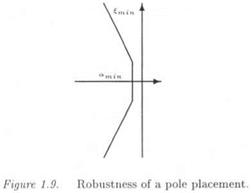
ft may be the unit disc in the case of discrete time systems, or a trun­cated sector in the continuous-time one (see Figure 1.9). Performance is indeed defined in this context by minimal values £TOjn and amm for the damping ratio £ and the degree of stability a [4]. To some extent, these specifications correspond to requirements on the rise time and overshoot of the closed loop step response, or on the time needed to reject an unmeasured disturbance or a non zero initial condition.