Scaling of the Radiation-Adiabatic Temperature

The radiation-adiabatic temperature is, in contrast to the recovery tempera­ture, Reynolds number and scale dependent, Sub-Section 3.2.1. Therefore, data from different cases, even with the same total enthalpy, cannot di­rectly be compared. The radiation-adiabatic wall temperature on a small body (wind-tunnel model) would be much larger than that on a large one (real configuration), if all flow parameters are the same. This makes a full simulation in an hypothetical ideal wind tunnel impossible. This holds also for an experimental or demonstrator vehicle, which could be a scaled-down version of the reference concept.

If in design work an input about the distribution of the radiation-adiabatic temperature is quickly needed, a scaling of it from another, already computed case, can be made. Precondition is that the flow topology qualitatively and quantitatively is the same in both cases (geometrical affinity, the same angles of attack and yaw), that it is not too strongly three-dimensional, and that (high-temperature) real-gas effects are similar. In addition, the assumption must be made that the recovery temperature Tr is constant over the entire vehicle surface (flat-plate behavior), although different for laminar and tur­bulent flow portions. This assumption, however, may be violated to a certain extent in reality, but without posing a serious restriction for the use of the following scaling laws.

If the two different cases 1 and 2 are considered, we obtain with eq. (3.25)

which does not depend on x/L, i. e., it holds for every point on the surface, if Tr if sufficiently constant. Of course the respective portions on the vehicle surface with laminar flow (scaling with n = 0.5) and with turbulent flow (scaling with n = 0.2) must be the same in case 1 and 2. If the flow is fully laminar (RV’s above 40-60 km altitude) this is no problem. At the flight of a vehicle of either vehicle class below that altitude, one must be aware that this should hold at least approximately. If that is not the case, one has to make sure that is does not seriously curtail the result.

1 (ДеГЄ/,ь)і~П L2 Trl 1 {Reref, L)l2 11 ^1 Tr2

If Tra is small compared to Tr in both cases, eq. (3.33) can be reduced to

Eq. (3.33) can be written in terms of the unit Reynolds number Reu =

pre fvref /M ref •

re/)l " L72 Tr 1 (1 — Tra/Tri)

With the formulations given in Sub-Section 7.2.6 scaling relations can be derived also for stagnation point regions and attachment lines. All relations permit a wide range of parameters to be covered in the scaling process. All can be further reduced like above for unit Reynolds numbers etc.

The parameter variation range of a scaling law of this kind unfortunately cannot be firmly established from first principles. In design work it must be established for each given case before application.

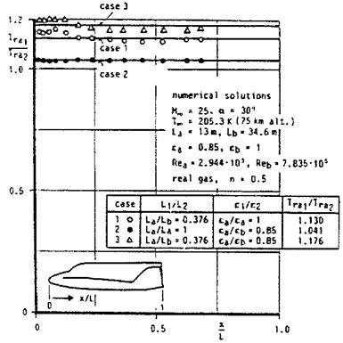
Figs. 3.10 and 3.11 demonstrate scaling—with a slightly modified eq. (3.34)—for the windward side of the HERMES configuration with laminar flow. Three cases were studied [33]. The numerical results were obtained with the coupled Euler/second-order boundary-layer method described in [14]. The flight conditions are given in Table 3.3.

Table 3.3. Flight parameters for the scaling of the radiation-adiabatic temperature at HERMES [33]. H [km] ТА [K] Reto [1/m] a [°] Boundary layer 25 75 205.3 0.2265-105 30 laminar

Case 1 scales the radiation-adiabatic temperature of HERMES with the original length La = 13 m with that of a HERMES configuration enlarged linearly to Lb = 34.6 m, the length of the Space Shuttle Orbiter. In case 2 a scaling is made on the original HERMES configuration for two different emissivity coefficients ea = 0.85 and eb = 1. In case 3 finally case 1 and case 2 are combined.

Fig. 3.10 shows at the windward side a rather good scaling with somewhat larger deviations in the nose region. There, of course, the simple flat-plate relation eq. (3.25) is only approximately valid. The expected very good scaling for case 2 shows slight deviations in the nose region, which are probably due to the non-linear coupling between the boundary-layer thickness and the radiation-adiabatic temperature.

The scalings in Fig. 3.11 for the lower side cross-section at x/L = 0.468 show larger deviations in the vicinity of the leading edge. Here, at the attach­ment line, which lies well at the lower side of the configuration, the original assumption in the scaling laws of a flat-plate boundary layer introduces larger errors. At an attachment line the flow is highly three-dimensional [18], which will be shown in the case study in Section 3.3.

Fig. 3.10. Comparisons of Trai/Tra2 at the lower symmetry line of HERMES [33]. Symbols: numerical results, full lines: scaled results.