AFFINE UNCERTAINTIES

Consider the case of parametric uncertainties Si entering in an affine way the state-space model of the plant:

N N

x = (Ao + Ai8i)x + (Bo + Bi8j)u

i=1 t=l

N N

У = (Со + £едя + (В0 + £Вгй)и (3-3)

i=l i=l

with dim x = n, dim n — — and dim у — —. The above equations can be rewritten as:

where (j €E [0, N]):

The idea is to introduce additional fictitious inputs and outputs w and z, so that the uncertainties <5г appear as an internal feedback w = Az, with Д = diag(5ilqi). To this aim, the following augmented model is introduced:

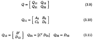
Matrices (^4о,-Bo, Co, Do) represent the nominal plant model (i. e. the one corresponding to 5 = 0). The issue is to look for matrices В’, C, Dyii A2i, £>22 and for a structured model perturbation Д satisfying (V «5 Є Rn):

The LFT Fi(Q, A) can be written as:

Fi(Q, A) = Qn + QnA(I – Q22A)~1Q2i

with:

Because of the affinity of the equations as a function of the parameters Su Q22 = 0. Matrices Q21 et Q12 must satisfy:

Let q, the rank of matrix =, which can be factorized as:

with P= q Pn’ =* , Pi q Pnq ’ =* , Pi q Pn• =* and Pi P Pn= ’ =• . As a con­

sequence:

It is then deduced that:

With reference to the above equation and to relations (3.11) and (3.12), one obtains by identifying each term:

B’ = [h… LN]

D2 = [Wi… WN]

C = [i? i… Rn]T

D21 = [Z … Zn]t

-D’22 = 0

Д = diag(dilqi) (3.16)

The issue is finally to come back to an input/output framework. Equa­tion (3.3) corresponds to a transfer matrix у = G(s, S)u, where as equa­tion (3.6) corresponds to the augmented transfer matrix:

As expected, when using the feedback = = P z, one obtains:

y = G(s,6)u = Ft(H(s),A)u (3.18)