Continuous-Time Model

Let a system be described by a linear constant coefficient, ordinary n-order differ­ential equation:

dny(t)/dtn + я„_1 dn Vf)/df” 1 +———– h a0y(t)

= tp dpu(t)/dtp + ••• + r0u(t) (2.1)

Here, u(t) is the system input and y(t) its output. Taking the Laplace transform [2], and assuming that the initial conditions are zero, we obtain the continuous-time TF (CTTF):

y(s) = G(s) u(s)

Tpsp + tp—1 S’-1 h – h t1s + t0 (2:2)

= u(s)

sn + an-1sn 1 + ••• + a1 s + a0

Here, s is a complex (frequency) variable. This is one type of the mathematical model of a SISO system. The linear theory of analysis can be applied to this model and the system’s properties can be analytically derived from this model itself. The natural dynamic behavior of the system, in fact now of the model, can be evaluated by computing the roots of the denominator of G(s). These roots describe the various natural modes of the system, assuming that the model is nearly a good representation of the system, and dictate the amplitude and the phase of the response. If the value of n is equal to 2 then this TF is called a second-order TF and its denominator has two roots (real/complex). One can relate this to short-period modes of an aircraft wherein the short-period frequency and damping are important parameters, which are often discussed in dealing with simulation/control of aircraft (Chapter 5). These frequency and damping parameters in turn depend on certain important aerodynamic (stability and control) derivatives of the aircraft, the description of which is given in Chapter 4.

Example 2.1

Obtain the Bode diagrams for the TF of an electrical circuit of Figure 2.3 for the time

constant of 0.1 and 0.5 s. The resistor is R Ohm and the capacitance is C microfarad.

The time constant is given as RC = t(s).

Solution

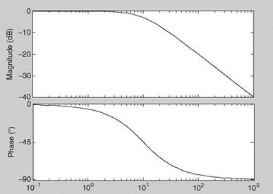
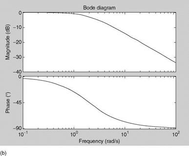
Specify numerator and denominator of the TF as num = [10], den = [1 10] (in the command window of MATLAB). Then use sys = tf(num, den) and bode(sys) to obtain/plot the Bode diagram (Figure 2.4). Repeat with 10 replaced by 2. At the cutoff

(a)

FIGURE 2.4 (a) Bode plot of the first order continuous-time system with t = 0.1 s. (b) Bode plot of the first order continuous-time system with t = 0.5 s.

FIGURE 2.5 Mechanical spring-mass system.

frequencies (Cof, cutoff frequency = 1/time constant) the phase (lag) is —45°, the property of the first-order TF. The bandwidth (Appendix C) of the system with Cof = 10 rad/s is broader than that with Cof = 2 rad/s.

Example 2.2

The TF of a second-order mechanical system of Figure 2.5 is given as

G(s, Xs) = K/M

() f (s) s2 + (D/M)s + K/M

Here, M is the mass, D is the damping constant, and K is the spring stiffness/constant. Use suitable values for M, D, and K and obtain the Bode diagrams. Study the improvement in the damping property by increasing the value of D by a factor of 2.

Solution

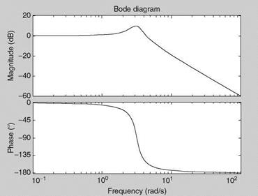
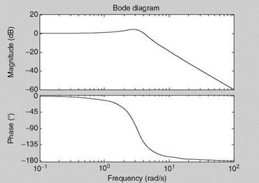
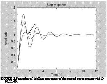
Let M = 10, D = 10, and K = 100, arbitrarily. Obtain numerator and denominator of the TF as num = [10], den = [1 10/10 100/10]. Then use sys = tf (num, den) and bode(sys) to obtain=plot the Bode diagram. We see that the natural frequency is sqrt(K/M) = 3.1623 rad/s and the damping ratio = 0.1581 (of the second-order system; Exercise 2.2), which is not the same as the damping constant. Due to low damping the magnitude of the TF has a peaking value (Figure 2.6a). Repeat the solution with D = 20 (Figure 2.6b). The increased damping constant has increased the damping ratio (the magnitude of the peak is reduced). The step responses are improved (Figure 2.6c). The step response is generated by step(sys). The first plot is held (by typing ‘‘hold’’) and then the step response with D = 20 gets automatically superimposed. We see that the time response is still not damped well. With D = 40 the response (with arrow) is very well damped and acceptable. The time constant (Appendix C) is approximately the same but the transients are suppressed when the value of D is increased. One can easily relate this TF to the short-period mode of an aircraft (Chapter 5). Thus, in the (very) approximate sense, the aircraft’s pitching motion dynamics are like a second – order spring-mass system.

Example 2.3

Obtain the Bode diagrams and the step responses of the following TFs [11] and comment on the results.

Solution

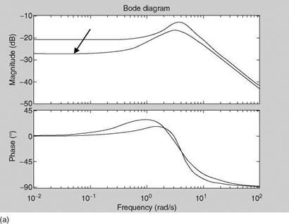
First, we obtain the Bode diagrams by using the steps: numl = [0.787 1.401]; deni = [1 3.785 15.49]; sysl = tf(numi, deni); bode(sysl); hold; num2 = [0.638 0.451]; den2 = [1 4.67 10.30]; sys2 = tf(num2,den2); bode(sys2) (in this sequence in the MATLAB command window). The plots are shown in Figure 2.7a. Then, we

(a)

(b) FIGURE 2.6 (a) Bode plot of the second-order continuous-time system with D = 10. (b) Bode plot of the second-order continuous-time system with D = 20.

(c)

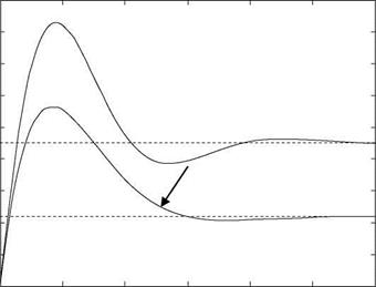
obtain the step responses by using step(sys1); hold; step(sys2) (the plots are shown in Figure 2.7b). Next, we obtain the poles of these TFs: roots(den1) — —1.8925 ± 3.4509; roots(den2) — —2.3350 ± 2.2018. We also have the damping ratios and frequencies as

FIGURE 2.7 (a) Bode plots of the second-order systems (sys1; sys2 with an arrow).

(continued)

0 0.5 1 1.5 2 2.5 3 Time (s)

(b)

FIGURE 2.7 (continued) (b) Step responses of the second-order systems (sysl; sys2 with an arrow).

damp(sys1) = 0.481, 3.94; damp(sys2) = 0.728, 3.21. We see that the second system has much better damping than the first one as is obvious from the step response of the second system (Figure 2.7b; see arrow). Actually these TFs/models are the lower-order equivalent system models (LOTF in Chapter 10) of the pitch rate to longitudinal input of F-18 HARV (high angle of attack research vehicle), identified from the measured data [11]. These LOTF models are used for evaluation and prediction of the HQs of the aircraft (Chapter 10).