Shocks
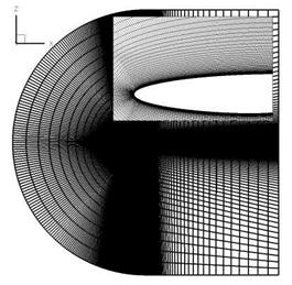
The correct prediction of flows with high pressure gradients, especially at shocks, also varies with the choice of the turbulence model, both in position and intensity. This again leads to changing values of lift and drag. For the investigation of this influence the 2D test-case RAE 2822 case 9 (Re = 6.5e6, Ma = 0.73) with a = 2.8 angle of attack and a shock at 55% chord length was applied. The grid is fully structured and consists of 200,000 grid points (fig. 13). It has an orthogonal wall resolution and a highly resolved boundary layer to exclude influences of errors. To achieve a more universal forecast for the computation of the shock position variations of the angle of attack (a = [1.0deg, 3.2deg]), the Mach number (Ma = [0.72…0.76]) and Reynolds number (Re = [6.0 • 106…107]) were investigated.
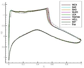
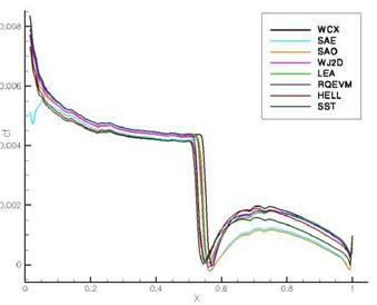
The variation of the turbulence models leads to visible variations in the shock position and the level of the cp and Cf coefficients (fig. 14 & 15). In comparison to the experiment the lift coefficient differs up to 4.6% and the drag coefficient up to 8.9% (e. g. Hellsten). The range between the models is +/ – 3.33% in the lift,
|
Fig. 13 Grid of the RAE 2822 test-case with 200,000 grid points |
|
Fig. 14 RAE 2822 case9 — pressure coefficient Cp in comparision with the eight different turbulence models and the experiment |
+/ — 7.55% in the drag coefficient and +/ — 2.86% in the shock position around the average of the results. There are obvious dependencies on the choice of the turbulence model and the shock position correlates very well with the lift coefficient. The results have shown that in the most investigated test-cases the prediction of
|
Fig. 15 RAE 2822 case9 — friction coefficient Cf in comparision with the eight different turbulence models |
|
Table 2 RAE2822 case9 – lift and drag coefficient, shock position compared to experimental results
|
the shock position correlates with the turbulence model (left-hand side, fig. 16). In cases where another uncertainty exists, for example a separation bubble, (right-hand side, fig. 16, divergent progress) there is no exact forecast possible for the model dependency. Because of the unchanged order of the models a user feedback that shows only tendency is still possible.
1,060E+0 1.055E+0 1.050E+0 1.045E+0 1.040E+0 1.035E+0 1.030E+0 1.025E+0 1.020E+0 1.015E+0 1.010E+0 1.005E+0 1.000E+0 9.950E-1 9.900E-1 9.850E-1 9.800E-1 9.750E-1 9.700E-1 9.650E-1 9.600E-1 9.550E-1 9.500E-1
![]()
![]() Fig. 16 RAE 2822 case9 — Position of the compression shock normalized by the position of the SAE model with variations of Mach number, Reynolds number and angle of attack
Fig. 16 RAE 2822 case9 — Position of the compression shock normalized by the position of the SAE model with variations of Mach number, Reynolds number and angle of attack
Implementation of the Shock Sensor
To detect a compression shock all grid elements were scanned of characteristic physical values and marked if they exceed a given limit. These values are high pressure gradients in flow direction and a Mach numbers near 1. By projection of the normalized pressure gradients on the velocity a factor for the relative pressure increase was achieved and should come to 30%. The deviation of the Mach number from 1 should be less than 5%. These limits can be adjusted in the TAU solver butrepresent in all investigated test-cases very good indicators for a shock. The marked areas are available as an output value in the TAU routines.


