NUMERICAL APPROXIMATIONS — REDUCTION OF INTEGRAL EQUATIONS INTO MATRIX EQUATIONS

In practical numerical calculations, the integral equations of the pre­ceding sections can be replaced by matrix equations. As a physical * Sometimes also called latent roots, or eigenvalues.

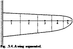
example, consider the divergence of the cantilever wing shown in Fig. 3.4. In analyzing the wing deformation approximately, it is natural to divide the wing into a number of segments. The loading on each segment may be assumed as concentrated at a reference point in the segment. The average angle of rotation in each segment is represented by that measured at the reference point. Let ві be the angle of rotation of the ith segment, and Mt the aerodynamic moment in the same. Let the influence coefficient

у

for rotation at the rth segment due to a unit moment at the y’th segment be denoted by ctj. Then the total rotation at і is obtained by summing over the effects of all the moments:

(1)

where n is the total number of segments in which the wing is divided. It is convenient to write в{ and Mt as matrices в and M:

Then Eq. 1 can be written simply as

9 = c • M or {0J = {cw}{M,} (4)

M is a linear function of 6 and is proportional to the dynamic pressure q. Hence, we may write, in general,

M = #A • 9 (5)

{M^ = q{AM}

where {Ah} is a square matrix. The form of the matrix A depends on the aerodynamic theory used (cf. § 4.5). In particular, if the “strip” assumption is used, A becomes a diagonal matrix:

where a is the lift-curve slope, c{ the chord length at the /th segment, and ег the eccentricity, i. e., the ratio of the distance between the aerodynamic center and the elastic axis at the /th segment to the chord length. The condition of divergence can be represented as

9 = qAivc • A • 9 (7)

from which the eigenvector 0 and the eigenvalue q can be solved. An example will be given in § 4.5. Equation 7 should be compared with Eq. 3 of §3.2.

That all the methods discussed so far can be transformed into matrix form is evident from recognizing that the matrix formulation amounts to a finite-differences approximation of continuous operations. We represent a continuous function Y(x) of x in the interval (a, b) by a numerical table:

X	a = x0	Xl	x2		Xn = b
Y(x)	Yo	Y,	Y2		Yn

If the divisions (xj — Xf_j) are sufficiently fine, this table will represent sufficient information for the function Y(x). The value of Y(x) at a point x other than the x-s can be obtained by interpolation.3-21"3 2"

By using the method of finite differences, the derivatives and integrals of Y(x) can be replaced by a suitable combination of Y(x{), and equations governing Y(x) can be written as matrix equations with Y(x{) as elements. From a mathematical point of view, the introduction of finite differences to replace continuous differential and integral operators is an approximation

whose convergence can be rigorously treated. From an engineering point of view, the finite-differences method is the only natural method of specifying any physically measurable quantities. For example, in order to record the deflection curve of a beam under certain specified loading condition, the best an engineer can do is to measure the deflection at as many stations as possible. The result is a numerical table of the deflection function.

An integral is approximated as follows. Let Y(x) be given at the points xm = — (b — a) (m — 0, 1, • • •, n), the points xm being equally spaced. Let us write

Y(xJ = Ym

(8)

The “weights” sm are taken from the well-known rules of integration. For example,

	Sq Si ^2 ‘	Sn-2 $п—1 ^Vi
1. Trapezoid rule	і 1 1 1 •	• 1 1 і
2. Simpson’s rule (я, even)	1 4 2 4-	• 2 4 Ї

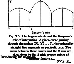
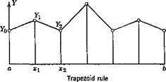
There are other more complicated rules which, however, are often inferior to the simple rules quoted above, save for exceptional cases. Represented graphically, these rules are illustrated in Fig. 3.5. Equation 8 can be written as a matrix product

fy(x)dx = hsY (9)

Ja

where Y is a column matrix, s is a row matrix of “weights,” and h is a constant:

Y0

Yi

Similarly, a function of two variables K(x, y) can be represented as a double-entry table. Let the domain of (x, y) be the square (a < x, у < b), and let the interval (a, b)2 be divided into n2 subdivisions by the points

Уо = а, yn = b

xo — at xl> ‘ " "> Xn—1* Xn — ^

(И) (12)

we may write

І’ЬК(х, у)ф{у)<іу = ЖБФ Ja

where

кп	• •	• к1п
Knl	Kn г	■ • кпп

Ф>

ft is gven by Eq. 10, and S is a diagonal matrix of “weights”:

The integral equation

ф(х) — A f K(x, уЩу) dy =f(x)

Ja

is then replaced by the approximate matrix equation

Ф – МКБФ = f

where f is a column matrix with elements (/г,/2, • • •,/„)■

The matrix equation 15 can be made a starting point for a rigorous treatment of integral equations. The mathematical theory has been completed by Volterra, Fredholm, Hilbert, and others.

In Eqs. 8, 9, and 12 it was assumed that the intervals between the sub­divisions (xt — xt_j) are equal. In some cases it is advantageous to use

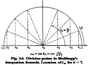
unequal subdivisions, such as in Gauss’s integration formula (cf. p. 159 of Ref. 3.21 or p. 115 of Ref. 3.23). However, in aeroelastic problems involving airplane wings, it is usually advantageous to use Multhopp’s

formula which emphasizes the wing-tip regions. Multhopp’s formula,4-51 as is known in the theory of lift distribution, is

This formula holds exactly so long as the function Y(x) can be represented by a series of the following form:

Clearly, with a suitable modification of the constants slt • • -, ^r„ the method of reducing an integral equation into a matrix equation remains the same for unequal subdivisions (cf. sections on “divided differences,” pp. 20, 96, 104, Ref. 3.21).

3.4 CONCLUDING REMARKS

Throughout this chapter the aerodynamic moments have been based on the “strip” assumption. Relaxation of this assumption leads to compli­cated equations. For a normal wing without appreciable sweepback angle, the over-all effect of finite-aspect ratio on the divergence speed can be accounted for by taking the lift-curve slope a corrected for aspect ratio.

The effect of compressibility can be included by using proper aero­dynamic coefficients which correspond to the Mach number at which divergence occurs. The calculation can be made by a process of trial and error.