SIMPLE METHOD FOR PHYSICAL MODELS
The aim of this section is to illustrate through a simple example a straightforward method, for introducing uncertainties in the plant model and obtaining the associated LFT model (see also the next chapter).
 |
Consider a real modal state-space model of a flexible plant. When focusing on a single flexible mode with damping ratio £ and natural frequency ш, one obtains:
Where the bf’s are row vectors, while C is a matrix. An uncertainty in the natural frequency w is introduced as:
![]() u> — (1 + 5)(Jo
u> — (1 + 5)(Jo
 where ujq denotes the nominal value and 6 the relative variation. The state-space model above becomes:
|
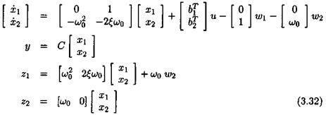
Fictitious input (vector) w and output (vector) z are introduced: |
|
|
Let Д = Sln. When applying the fictitious feedback w = Az, the issue is to determine the integer n and the state-space matrices В, C, D and ї>2, for which the state-space model of equation (3.31) reduces to the state-space model of equation (3.30).
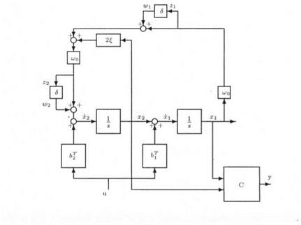
Figure 3.5. A physical method for introducing uncertainties in a plant model
This problem can be solved in an analytical way. However, an alternative very simple solution uses the physical representation of the state-space model (3.30): see Figure 3.5. The idea is to compute the augmented plant H(s) of Figure 3.5, with inputs u, w and w2 and outputs y z and z2 (and 5 = 0):
|
|
Let Д = diag( 5, 5 ) . The LFT transfer Hi ( H( s) , Д ) coincides with the transfer (3.30) between input u and output y, and this LFT realization is minimal.


