Our heavyweight helicopter equal in the world does not have
In Rostov started production of the most load-lifting rotary-wing car The Russian holding «Helicopt[...]

Everything about aircrafts and helicopters. News and events in aviation worldwide. Civil, transportation, military helicopters and airplanes.

Everything about aircrafts and helicopters. News and events in aviation worldwide. Civil, transportation, military helicopters and airplanes.

Everything about aircrafts and helicopters. News and events in aviation worldwide. Civil, transportation, military helicopters and airplanes.

Everything about aircrafts and helicopters. News and events in aviation worldwide. Civil, transportation, military helicopters and airplanes.


How best to transform a boundary value problem governed by partial differential equations into a computation problem governed by difference equations is not always obvious. The task is even more difficult if the original problem involves a surface of discontinuity. There is a lack of discussion in the literature about how to model a discontinuity in the context of finite difference. The purpose of this section is to show how one such model maybe set up. At the same time, this model will demonstrate that the finite difference formulation of boundary value problems may support spurious boundary modes. These modes might have no counterpart in the original problem.
![]()
|
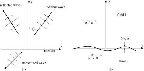
They are not generally known or expected. If one of these spurious boundary modes grows in time, then this could lead to numerical instability or a divergent solution. Consider the transmission of sound through the interface of two fluids of densities p(1) and p(2) and sound speeds a(1) and a(2), respectively, as shown in Figure 1.4a. It is known that refraction takes place at such an interface. Superscripts (1) and (2) will be used to denote the flow variables above and below the interface. For small-amplitude incident sound waves, it is sufficient to use the linearized Euler equations and interface boundary conditions. Let y = g(x, t) be |
|
the location of the interface. The governing equations are du(1) 1 9 p(1) |
|
d v(1) |
|
9 y (1) 9 u(1) 9 v(1) P 1 — + -9У = 0 |
|
y = 0, p(1) = p(2) (1.44) ^ = v(1) = v(2). (1.45) |
|
|
 |
![]()
For static equilibrium, the pressure balance condition is
![]() p(1) = p(2) or P(1)(fl(1)}2 = P(2)(fl(2)}2.
p(1) = p(2) or P(1)(fl(1)}2 = P(2)(fl(2)}2.