Computation Models
For the computation of equilibrium or non-equilibrium flows different air models are available. If ionization, Section 2.1, can be neglected, one can work with the five species (N2, O2, N, O, NO) model with 17 reactions. If ionization is to be taken into account, the eleven species model with 33 reactions, [7], can be employed. In this section we give some references to literature on detailed computation models for the thermo-chemical and transport properties of air in the temperature and density/pressure range of interest for both thermo-chemical equilibrium and non-equilibrium flow, see also [6].
Equilibrium Flow. The transport properties of air can be determined with the models presented in Chapter 4. Characteristic data for thermo-chemical properties can be found, e. g., in [7], and for transport properties in [29]-[32]. Regarding the general state of the art, including modeling problems, we refer to the review paper [9].
|
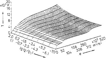
Fig. 5.14. State surface of the temperature T of equilibrium air as function of the density p and the internal energy e [36]. Database: [33] to [35] (p0 = 1 kg/m3). |
It is recommended to work in computation methods with state surfaces of thermodynamic and transport properties, because their use is computationally more efficient than that of basic formulations. As was mentioned in Sub-Section 4.2.5 such state surfaces are available in the literature, e. g., [33] (only up to 6,000 K), [34, 35].
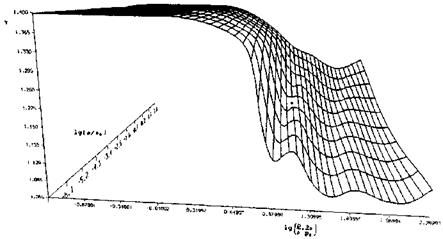
In [36] approximations of such state surfaces are given. We show as example in Fig. 5.14 the temperature T as function of the two variables density p (here in the form lg(p/po)), and internal energy e, and in Fig. 5.15 the ratio of specific heats 7 as function of lg(p/po) and lg(pp0/pp0). Note that van der Waals effects, Section 5.1, are not included.
Examples of state surfaces of the viscosity and the thermal conductivity are given in Sub-Section 4.2.5.
|
Fig. 5.15. State surface of the ratio of specific heats 7 of equilibrium air as function of the density p and the ratio pressure/density р/р [36]. Database: [33] to [35] (p0 = 1.292 kg/m3, po = 1.0133-106 Pa). |
Non-equilibrium Flow. Flows with thermo-chemical non-equilibrium must be modeled with the help of the basic formulations. Characteristic data again can be found, e. g., in [7] and [11]. We refer also to the review paper [9] regarding the general state of the art, including modeling problems.
Transport properties are treated like in equilibrium flow by taking into account the momentarily present thermo-chemical state of the gas with appropriate formulations, Sub-Section 4.2.5.
Special regard must be given to the boundary conditions of the species continuity equations, if finite catalytic surfaces are to be modeled. In [19], for instance, we find the formulations for the five and the eleven species gas model, and also general slip-flow boundary conditions.
5.3 Problems
Problem 5.1. A gas has the ratio of specific heats 7 = 1. Show that this is equivalent to f = to.
Problem 5.2. The reservoir enthalpy of a ground-simulation facility with air as test gas is ht = 20 MJ/kg. What are a) the maximum possible speed and the Mach number at the exit of the nozzle, b) the speed and the Mach number, if the static temperature at the nozzle exit is Texit = 1,000 K (assume a Lighthill gas at the exit), c) the speed and the Mach number, if in addition 20 per cent of the reservoir enthalpy is frozen? d) What is the general result?
Problem 5.3. The stagnation temperature is the temperature at the stagnation point of a blunt body. For inviscid flow it is the total temperature Tt. A CAV is approximated by a flat plate and flies with v= 2 km/s at 30 km altitude. What is a) Tt, if we assume 7 = 1.4 throughout? What is Tt, if we mimic high-temperature real-gas effects with b) Yeff = 1.3, and c) with Yeff = 1.1? d) What y is in a realistic range?
Problem 5.4. How does the uppermost curve of q in Fig. 5.11 scale with the ж-dependence indicated in eq. (3.27)? The result in Fig. 5.11 was obtained for a constant wall temperature, eq. (3.27) holds for a constant wall temperature, too. Measure q at ж = 1 m, and compare with the measured value at ж = 6 m.


