Modelling Helicopter Flight Dynamics

A mathematical description or simulation of a helicopter’s flight dynamics needs to embody the important aerodynamic, structural and other internal dynamic effects (e. g., engine, actuation) that combine to influence the response of the aircraft to pilot’s controls (handling qualities) and external atmospheric disturbances (ride qualities). The problem is highly complex and the dynamic behaviour of the helicopter is often limited by local effects that rapidly grow in their influence to inhibit larger or faster motion, e. g., blade stall. The helicopter behaviour is naturally dominated by the main and tail rotors, and these will receive primary attention in this stage of the Tour; we need a framework to place the modelling in context.

The problem domain

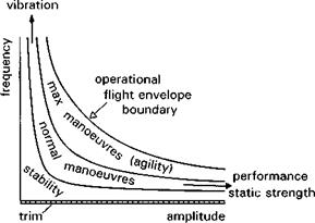
A convenient and intuitive framework for introducing this important topic is illustrated in Fig. 2.14, where the natural modelling dimensions of frequency and amplitude are used to characterize the range of problems within the OFE. The three fundamentals of flight dynamics – trim, stability and response – can be seen delineated, with the latter expressed in terms of the manoeuvre envelope from normal to maximum at the OFE boundary. The figure also serves as a guide to the scope of flight dynamics as covered in this book. At small amplitudes and high frequency, the problem domain merges with that of the loads and vibration engineer. The separating frequency is not distinct. The flight dynamicist is principally interested in the loads that can displace the aircraft’s

flight path, and over which the human or automatic pilot has some direct control. On the rotor, these reduce to the zeroth and first harmonic motions and loads – all higher harmonics transmit zero mean vibrations to the fuselage; so the distinction would appear deceptively simple. The first harmonic loads will be transmitted through the various load paths to the fuselage at a frequency depending on the number of blades. Perhaps the only general statement that can be made regarding the extent of the flight dynamicists’ domain is that they must be cognisant of all loads and motions that are of primary (generally speaking, controlled) and secondary (generally speaking, uncon­trolled) interest in the achievement of good flying qualities. So, for example, the forced response of the first elastic torsion mode of the rotor blades (natural frequency 0(20 Hz)) at one-per-rev could be critical to modelling the rotor cyclic pitch requirements correctly (Ref. 2.8); including a model of the lead/lag blade dynamics could be critical to establishing the limits on rate stabilization gain in an automatic flight control sys­tem (Ref. 2.9); modelling the fuselage bending frequencies and mode shapes could be critical to the flight control system sensor design and layout (Ref. 2.10).

At the other extreme, the discipline merges with that of the performance and structural engineers, although both will be generally concerned with behaviour across the OFE boundary. Power requirements and trim efficiency (range and payload issues) are part of the flight dynamicist’s remit. The aircraft’s static and dynamic (fatigue) structural strength presents constraints on what can be achieved from the point of view of flight path control. These need to be well understood by the flight dynamicist.

In summary, vibration, structural loads and steady-state performance traditionally define the edges of the OFE within the framework of Fig. 2.14. Good flying qualities then ensure that the OFE can be used safely, in particular that there will always be sufficient control margin to enable recovery in emergency situations. But control margin can be interpreted in a dynamic context, including concepts such as pilot-induced oscillations and agility. Just as with high-performance fixed-wing aircraft, the dynamic OFE can be limited, and hence defined, by flying qualities for rotorcraft. In practice, a balanced design will embrace these in harmony with the central flight dynamics issues, drawing on concurrent engineering techniques (Ref. 2.11) to quantify the trade-offs and to identify any critical conflicts.