Coefficients of Several Large Optimized Stencils

In this section, the coefficients of several large optimized stencils are provided. The range of optimization in wave number space is aAx = n.

9- Point Stencil

П = 1.28, a0 = 0.0

al = —a-1 = 0.8301178834769906875382633360472085 a2 = — a—2 = —0.23175338776901819008451262109655756 a3 = —a—3 = 0.05287205020483696423592156502901203 a4 = — a—4 = —6.306814638366300019250697235282424E-3

11-Point Stencil

П = 1.45, a0 = 0.0

ax = —a—1 = 0.8691451973307874495001324546317289 a2 = — a—2 = —0.28182159562075193452800172953580692 a3 = —a—3 = 0.08707110821545964532454798738037454 a4 = —a—4 = —0.019510858728038347594594712914321635 a5 = —a—5 = 2.265620835298174792121178791209576E-3

13-Point Stencil

П = 1.63, a0 = 0.0

al = —a—1 = 0.897853870484230495572085208841816 a2 = —a—2 = —0.32269821467978701682118324993041657 a3 = —a—3 = 0.12096287073505875036103692011036235 a4 = —a—4 = —0.037989102193448210970017384251701696 a5 = —a—5 = 8.526107608989087816184470859634284E-3 a6 = —a—6 = —1.0033637668308847022803811005724351E-3

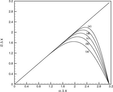
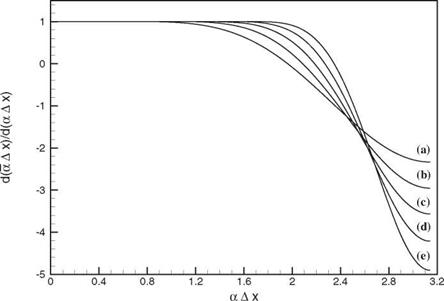
The a Ax versus aAx curves of these stencils are shown in Figure 2.11. Figure 2.12 shows the variation of the slope ^Ax) versus aAx. Figure 2.13 shows an enlarged portion of Figure 2.11 near the maxima of the curves.

Figure 2.11. The a Ax versus a Ax curves. (a) 7-point stencil, (b) 9-point stencil, (c) 11-point stencil, (d) 13-point stencil, (e) 15-point stencil.

Figure 2.12. The slope of the a Ax versus a Ax curves of Figure 2.11.

0.995

EXERCISES

2.1. Dimensionless variables with respect to length scale = Ax, velocity scale = c (speed of sound), and timescale = Ax/a are to be used.

Find the exact solution of the simple convective wave equation

d U d U

+ = 0 d t dx

Note that the entire solution propagates to the right at a dimensionless speed of unity.

Discretize the x derivative by the 7-point optimized finite difference stencil. Solve the initial value problem computationally. You may use any time marching scheme with a small time step At. Demonstrate that the numerical solution separates into two pulses. One pulse propagates to the right at a speed nearly equal to unity. The other pulse, composed of high wave numbers, propagates to the left. Explain why the solution separates into two pulses. Find the speed of propagation of each pulse from the j(aAx) versus a Ax curve and compare with your computed results.

2.2. Solve the following initial value problem computationally on a grid with Ax = 1

d U d U

+ = 0. dt dx

u (x, 0) = e ax cos (px)

Use the standard sixth-order central difference scheme.

Take a = 0.035 and consider three cases:

1. д = 0.8

2. д = 1.6

3. д = 2.1

For each case, plot u (x, t) at t = 300 and compare with the exact solution. Explain your results.

2.3. Solve the initial value problem:

— + — = 0 at t = 0, u = H(x + 50) – H(x — 50), dt dx

computationally on a grid with Ax = 1 , where H (x) is the unit step function,

Plot u(x, t) at t = 300. Determine from your numerical solution

(a) the most negative wave velocity (waves propagating to the left)

(b) the wave number of the wave with zero group velocity Compare the wave speed and wave number of (a) and (b) with the values from the ^ curve.

Do the above using

(1) the standard sixth-order central difference scheme and

(2) the optimized scheme (7-point stencil optimized over —1.1 < a Ax < 1.1).