Longitudinal Modes of a Jet Transport

The foregoing theory is now illustrated by applying it to the Boeing 747 transport. The needed geometrical and aerodynamic data for this airplane are given in Appendix E. The flight condition for this example is cruising in horizontal flight at approxi­mately 40,000 ft at Mach number 0.8. Relevant data are as follows:

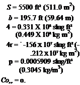
W = 636,636 lb (2.83176 X 106 N) c = 27.31 ft (8.324 m)

4 = 0.183 X 108 slug ft2 (0.247 X 108 kg m2) /z = 0.497 X 108 slug ft2 (0.673 X 108 kg m2) u0 = 11A fps (235.9 m/s) 0O = 0 CU) = 0.654

The preceding four inertias are for stability axes at the stated flight condition. In the numerical examples of this and the following two chapters, the system matrices and the solutions are all given in English units. The nondimensional stability derivatives

are given in Table 6.1, and the dimensional derivatives in Table 6.2. With the above data we calculate the system matrix A for this case. (Recall that the state vector is [Ли w q Д0]7). r

The characteristic equation (6.1,6) is next calculated to be:

A4 + 0.750468A3 + 0.935494A2 + 0.0094630A + 0.0041959 = 0 (6.2,2)

The two stability criteria are

E = 0.0041959 > 0 and R = 0.004191 > 0

so that there are no unstable modes.

EIGENVALUES

The roots of the characteristic equation (6.2,2), the eigenvalues, are Mode 1 (Phugoid mode): 2 = —0.003289 ± 0.06723г

Mode 2 (Short-period mode): A34 =—0.3719 ± 0.8875/ ^

We see that the natural modes are two damped oscillations, one of long period and lightly damped, the other of short period and heavily damped. This result is quite typ-

Table 6.2 Dimensional Derivatives—B747 Airplane X(lb) Z(lb) M(ft-lb) M(ft/s) -1.358 X 102 -1.778 X 103 3.581 X 103 w(ft/s) 2.758 X 102 -6.188 X 103 -3.515 X 104 <7(rad/s) 0 -1.017 X 105 -1.122 X 107 vv(ft/s2) 0 1.308 X 102 -3.826 X 103 ад Z(N) M(m-N) u(m/s) -1.982 X 103 -2.595 X 104 1.593 X 104 w( m/s) 4.025 X 103 -9.030 X 104 -1.563 X 104 </(rad/s) 0 -4.524 X 105 -1.521 X 107 vv(m/s2) 0 1.909 X 103 -1.702 X 104

Table 6.3 Period half Nhalf Mode Name (s) (s) (cycles) 1 Phugoid" 93.4 211 22.5 2 Short-period 7.08 1.86 0.26 "The phugoid mode was first described by Lanchester (1908), who also named it. The name comes from the Greek root for flee as in fugitive. Actually Lanchester wanted the root for fly. Appropriate or not, the word phugoid has become established in aeronautical jargon.

ical. The modes are conventionally named as in Table 6.3, which also gives their peri­ods and damping. The transient behavior of the state variables in these two modes is displayed in Fig. 6.2.