One-Dimensional Test Setup

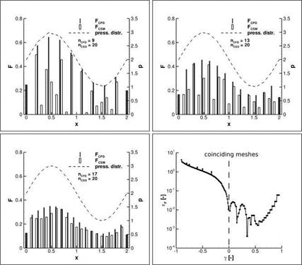
First investigations were carried out with one-dimensional test configurations loosely following an approach laid out by Jaiman et al. [17]: The one-dimensional fluid mesh and the structural mesh are colinear, but feature non-matching discretisations. An analytical pressure distribution is applied to the fluid mesh. The equivalent con­sistent nodal loads are then projected on the structural nodes. Furthermore, a refer­ence load distribution can be obtained by calculating the nodal loads consistent with the pressure distribution directly at the structural nodes. The reference loads can then be used to calculate a relative error eF of the projected loads. In the first three diagrams of Fig. 6, the analytical pressure distribution is plotted over the length of the one-dimensional domain together with the forces acting on the fluid nodes and on the structural nodes. The fluid mesh is discretised with an increasing number of elements nCFD, whereas the number of elements on the structural side is kept con­stant at nCSD = 20. In this example, linear shape functions are used for both the cal­culation of the consistent nodal forces and for their projection with the FIE method. With the coarser CFD meshes the distribution of the projected forces on the struc­tural nodes is highly irregular. Parameter studies indicate that the mesh spacings on

both sides have to be fairly similar in order to achieve a sufficiently regular load dis­tribution. The graph on the bottom right of Fig. 6 underscores this result. It shows the relative error plotted over the mesh ratio у = i+^csD/wcro’ Values from -1 to 0 imply a fluid mesh coarser than the structural mesh, and values between 0 and 1 a finer one. For negative values of у the error is high, and only approaching у = 0 it decreases to an acceptable level. In this example, for у = 0 the structural nodes and the fluid nodes are placed at the same coordinates and the relative error becomes zero (not shown in the logarithmic diagram).