Wind-Tunnel Models

In this section, we consider three types of mounting for wind-tunnel models: wall – mounted, sting-mounted, and strut-mounted. Expressions for the aeroelastic pitch deflections are developed for these simple models that, in turn, lead to a cursory understanding of the divergence instability. Finally, we briefly return to the wall – mounted model in this section to consider the qualitatively different phenomenon of aileron reversal. All of these wing models are assumed to be rigid and two­dimensional. That is, the airfoil geometry is independent of spanwise location, and the span is sufficiently large that the lift and pitching moment do not depend on a spanwise coordinate.

4.1.1 Wall-Mounted Model

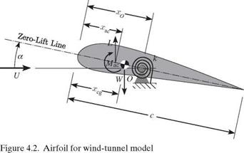
Consider a rigid, spanwise-uniform model of a wing that is mounted to the side walls of a wind tunnel in such a way as to allow the wing to pitch about the support axis, as illustrated in Fig. 4.1. The support is flexible in torsion, which means that it restricts the pitch rotation of the wing in the same way as a rotational spring would. We denote the rotational stiffness of the support by k, as shown in Fig. 4.2. If we assume the body to be pivoted about its support O, located at a distance xO from the leading edge, moment equilibrium requires that the sum of all moments about O must equal zero. Thus

Were the support rigid, the angle of attack would be ar, positive nose-up. The elastic part of the pitch angle is denoted by в, which is also positive nose-up. The wing angle of attack is then a = ar + в. In anticipation of using linear aerodynamics, we assume the angle of attack, a, to be a small angle, such that sin(a) « a and cos(a) « 1. It also is necessary to restrict the analysis to “thin” airfoils (i. e., small thickness to chord and small camber). The treatment herein is restricted to incompressible flow, but compressibility effects may be taken into account by means of Prandtl-Glauert corrections to the airfoil coefficients. For this, the freestream Mach number must remain less than roughly 0.8 to avoid transonic effects.

For linear aerodynamics, the lift for a rigid support is simply

^rigid = qSCLaar (4.2)

whereas the lift for an elastic support is

L = qSCia (ar + в) (4.3)

where q = 1 pmU2 is the freestream dynamic pressure (i. e., in the far field—often denoted by qTO), U is the freestream air speed, pTO is the freestream air density, S is the planform area, and CLa is the wing lift-curve slope. Note that L = L^d; for positive в, L > L-igid. We can express the moment of aerodynamic forces about the aerodynamic center as

Mac = qScCMac (4.4)

If the angle of attack is small, CMac can be regarded as a constant. Note here that linear aerodynamics implies that the lift-curve slope CLa is a constant. A further simplification may be that CLa = 2n in accordance with two-dimensional thin-airfoil theory. If experimental data or results from computational fluid dynamics provide an alternative value, then it should be used.

Using Eqs. (4.3) and (4.4), the equilibrium equation, Eq. (4.1), can be expanded as

qScCMac + qSCia (ar + в) (xo – xac) – W(xq – Xcg) = кв) (4.5)

Solving Eq. (4.5) for the elastic deflection, we obtain

qScCMac + qSCLaar (xo – xac) – W(xo – Xcg)

к – qSCLa (xo – Xac)

When ar and q are specified, the total lift can be determined.

When the lift acts upstream of point O, an increase in lift increases a that, in turn, increases lift. Thus, lift is a destabilizing influence counteracting the restraining action of the spring when xO > xac. Recalling the discussion of stability in Section 2.5, when a system is perturbed from a state of equilibrium and tends to diverge further from its equilibrium state, we say that the system is unstable. Such is the case when the moment of the lift about point o exceeds the restoring moment from the spring. This is one of the simplest examples of the static aeroelastic instability called “divergence.” Now, from Eq. (4.6), we see that the aerodynamic center is forward of the support point O when xac < xO, making it possible for the denominator to vanish or for в to blow up when q is sufficiently large. The denominator of the expression for в is a sort of effective stiffness, which decreases as q of increases. When the denominator vanishes, divergence occurs. The divergence dynamic pressure—or dynamic pressure at which divergence occurs—is then denoted by

к

SCia (xo – xac)

From this, the divergence speed—or the air speed at which divergence occurs—can be found as

It is evident that when the aerodynamic center is coincident with the pivot, so that xo = xac, the divergence dynamic pressure becomes infinite. Also, when the aerodynamic center is aft of the pivot so that xo < xac, the divergence dynamic pressure becomes negative. Because for physical reasons dynamic pressure must be positive and finite, it is clear in either case that divergence is impossible.

To further pursue the character of this instability, consider the case of a symmet­ric airfoil (CMac = 0). Furthermore, let xo = xcg so that the weight term drops out of the equation for в. From Eq. (4.7), we can let к = qDSCLa (xo – xac); therefore, в can be written simply as

в = iDrbi (4.9)

q

The lift is proportional to ar + в. Thus, the change in lift divided by the rigid lift is given by

a l = в = g

Lrigid ar 1 – qD

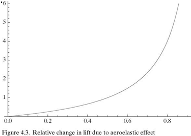
Both в and A L/L-igid clearly approach infinity as q ^ qD. Indeed, a plot of the latter is given in Fig. 4.3 and shows the large change in lift caused by the aeroelastic effect. The lift evidently starts from its “rigid” value—that is, the value it would have were
the support rigid—and increases to infinity as q ^ qD. However, remember that there are limitations on the validity of both expressions. Namely, the lift will not continue to increase as stall is encountered. Moreover, because the structure will not tolerate infinite deformation, failure takes place at some finite value of в—generally at a dynamic pressure well below the divergence dynamic pressure.

When the system parameters are within the bounds of validity for linear theory, another fascinating feature of this problem emerges. We can invert the expression for в to obtain

(4.11)

making it evident that 1/в is proportional to 1/q (Fig. 4.4). Therefore, for a model of this type, only two data points are needed to extrapolate the line down and to the left until it intercepts the 1/q axis at a distance 1/qD from the origin. As shown in the figure, the slope of this line also can be used to estimate qD. The form of this plot is of great practical value because estimates of qD can be extrapolated from data taken at speeds far below the divergence speed. This means that qD can be estimated even when the values of the model parameters are not precisely known, thereby circumventing the need to risk destruction of the model by testing all the way up to the divergence boundary.