4. A FURTHER STUDY OF THE и UPPER BOUNDS

• When comparing the two^ upper bounds in figures 9.1 and 9.2, the second и upper bound appears more conservative (at least in this ex­ample). Nevertheless, this conservatism remains quite reasonable: note especially that the two upper bounds are nearly identical around the peaks on the и plots, so that the robustness margin obtained with both upper bounds is nearly the same. This justifies to a large extent this second v upper bound, since it is easier to implement than the first v upper bound.

• In the example of Figure 9.2, the model perturbationAi (which is to be maintained inside its unit ball) contained two one-dimensional complex blocks, namely a fictitious performance block and a block of neglected dynamics. The scaling matrix G was consequently chosen as G — 0, while the scaling matrix D i was computed with the Perron eigenvector approach.

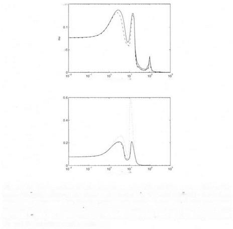
To further evaluate the methods of section 2.4 (chapter 8), anew mixed model perturbation Ai is chosen, which contains the fictitious perform­ance block, the neglected dynamics and two parametric uncertainties. Remember there are 4 parametric uncertainties in Ma, Za, Mg and Zg. In the lower subfigure of Figure 9.3, Ma and Za are included in the model perturbation Дi, i. e. the associated parametric uncertainties are 1This problem is very close to the problem of subsection 1.3 (chapter 6), the only difference being the full complex block which corresponds to the high frequency bending mode and which is not taken into account in chapter 6 (subsection 1.3).

to be maintained within ± 5 %. Conversely, in the upper subfigure of Figure 9.3, Ms and Z$ are included in

о ‘ і

Г’ о.

frequency m red » frequency n rad s

Figure 9.3. New problem of robust performance – Ms and Zs are expanded in the upper subhgure, where as Mn and Zn are expanded m the lower subhgure – the dashed dotted plot represents the first v upper bound, where as the dotted plot represents the second v upper bound without scaling matrices D and G (not shown in the upper subngure) – the two plots of the second v upper bound with scaling matrices

Dі and Gі are represented in solid line.

The following quantities are computed:

■ The first mixed и upper bound: this one is used as a reference.

■ The second mixed v upper bound with scaling matrices D = I and Gі = 0: the structure of the model perturbation Z i is not accoun­ted for. This upper bound is not presented in the upper subfigure of Figure 9.3, because of the bad results which were obtained: the assumption Z( Mi ) < 1 was not satisfied on many points of the fre-

quency gridding, so that the value of the upper bound was chosen as +oo on these frequency points.

The second mixed v upper bound with suboptimal scaling matrices D and G\ matrix G was computed with the suboptimal method by (Young et al., 1995), whereas matrix D i was computed using either the Perron eigenvector approach or Osborne’s method. The results provided by both methods are most generally equivalent. When com­paring with the first mixed v upper bound, the second mixed supper bound with suboptimal scaling matrices D and G appears more conservative, but this additional conservatism is quite reasonable.