Interpolation Quality Comparison

The different reduction algorithms in section 4.1 to 4.3 select different base point sets Xs from the input data site set Xinp. This section is comparing the resulting interpolation errors in a test case.

Therefore the extremely deformed half model airplane, as seen in figure 6 is used. The input base points Xmp and their deformation vectors AXmp were calculated with a structural loads program. The tool generates for each surface grid node a deformation vector, so the cardinality of Xmp and AXinp is quite large with a value of ninp = 137,136 for the wing without engine only.

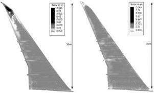
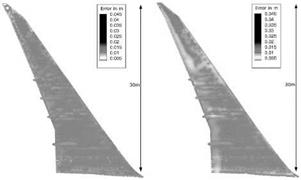
Figure 7 shows the interpolation error ei for the bottom surface of the wing, because it used to show higher interpolation errors. The settings for the interpolation and base point reduction can be seen in table 1.

Because the structural loads tool gives an deformation output for every surface grid node, the interpolation error for the surface nodes e = (ei)i=1 can be cal­

culated by taking the differences between the calculated interpolations AHi and the input deformations Axi:

Єі = \А% – Axi\2. (43)

The picture 7(a) clearly shows that the base points, chosen by the equidistant reduction method, are not satisfactory in the outer wing part. The outer 30 percent of the wing show strongly increased error values. This result has motivated to improve the base point selection process. The other reduction algorithms show a strongly improved interpolation error in this part of the wing, too. The mean absolute error ё of each test case for the actual 2000 base point setting, and additionally for another test series with only 1000 base points is given in table 2. Furthermore, this table contains the variance Var (e) and the maximal error max(ei).

i

The table confirms the impression of the given plots: All new methods choose base points resulting in a significantly lower interpolation error. Furthermore, the variance Var(-) indicates that less fluctuations in the error can be expected. The maximum error is lowered by up to 92 percent.

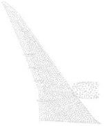
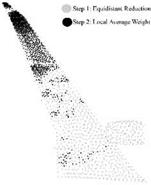
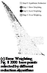
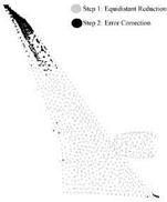
Figure 8 shows how the base points are chosen by the different algorithms. The equidistant reduction algorithm (7(a)) distributes the base points nicely over the whole domain. Taking a closer look, the decreased density of points in the thin parts of the wing, like the trailing edge and the tip, can be recognized.

Table 1 Test settings Reduction method Parameter RBF ф Equidistant reduction – Wendland’s C°, impact radius r = 20.0 Local average weighting fracequi = 0.5, dmin — dmaxiЮ Error weighting fraCeqm = 0.5, ^EWSteps = 3 Error correction fracequi = 0.5

(a) Equidistant Reduction	(b) Local Average Weighting

Table 2 Test results interpolation error e = (et)= n. (a) 1000 base points Reduction method e [m] Var(e) [m1] max(<?/) [m] І Equidistant reduction 5.30E-03 8.52E-02 1.24E-04 Local average weighting 1.56E-03 3.87E-02 3.83E-06 Error weighting 1.52E-03 1.10E-02 3.00E-06 Error correction 1.40E-03 8.99E-03 1.19E-06

(b) 2000 base points Reduction method e [m] Var(e) [m2] max (в/) [m] і Equidistant reduction 2.33E-03 2.52E-05 4.99E-02 Local average weighting 8.60E-04 1.92E-06 1.91E-02 Error weighting 6.86E-04 6.20E-07 7.92E-03 Error correction 7.38E-04 4.55E-07 3.83E-03

(a) Equidistant Reduction (b) Local Average Weighting

The new methods have all used the equidistant reduction algorithm in the first step for half of their base points. The remaining half has been selected differently, besides all algorithms concentrate the selected points in the outer wing part.

The local average method (8(b)) is the most extreme example for this behavior. Because the deformations are increasing with a parabolic character, the weights used to be more significant in the outer part. Supplementary, the more narrow getting wing supports this behavior, because the neighborhood of a certain point would contain more points of the side closer to the fuselage then from the outer side, which influences the local mean deformation.

The two remaining approaches based on the interpolation error are choosing their base points similarly. A difference between the error based greedy algorithms is that the error weighting algorithm is distributing the points more numerous in areas far away from the outer wing. The error correction algorithm has selected most points in the tip area.

The results show the best point selection for the error weighting and error cor­rection method. But one has to keep in mind that error correction is only working with radial basis functions with limited influence range, while error weighting has the larger computational costs (7 times larger than error correction).