Multivariate Interpolation Using Radial Basis Functions

The radial basis functions approach is a well-established interpolation method for gridded and scattered data, whereas the most natural context for function approxim­ation is given for scattered data [5, p. 99], [4, p. 4]. In the field of computational fluid dynamics (CFD) it is often used for coupling CFD-grids to finite element structure grids.

The input data in d dimensions consist of data locations xi, merged into the data­set

X = {X1,X2,…,Xn}e Rd, (1)

and the corresponding function values

fi = f(Xi) e R, i = 1,…,n. (2)

The data locations xi are called centers or "base points".

The goal is to interpolate the function values between the base points by an ap- proximant s : Rd ^ R to satisfy the condition

s|x = f x. (3)

In this specific case s is a linear combination of shifted radially symmetric basis functions ф. Radially symmetric means that the value of ф(-) depends only on the distance of the argument to the origin, hence it is often written ф (11 ■ 11). The distance norm is usually the Euclidean norm (with d = 3)

з (x) has the general form

3(x) = ^агф (Ух-x;||). (5)

i=1

Setting s(xi) equal to fi for all i n} leads to the linear system

Ay = b (6)

with

A unique interpolant is usually (for most ф) guaranteed, if the base points are all distinct and there are at least two of them [3, p. 6]. An example for a radial basis function could be ф (||x||) = ||x||2log ||x||, which is called "thinplate spline".

An important attribute of this interpolation method is the possibility to expand the approach of equation (5) by adding a polynomial to the definition without losing the uniqueness of the coefficients. For function values f, which show a polynomial character, the appended polynomial improves the interpolation quality. The only restriction is that the polynomial must have a degree m > 1 and is non-zero at all base points. This leads to:

n

s (x) = ф(||x – x!)+ p(x).

i=1

The coefficients can be computed by solving

n

s (x) = £a^(||x – x*||) + p(x)= fi (9a)

i=1

0 = ^atq (xi) V q: deg(q) < deg(p) (9b)

i=1

The extra equation (9b) takes up the extra degrees of freedom given by the poly­nomial coefficients, to allow a unique interpolant. The uniqueness can be guaran­teed, if ф is "conditionally positive definite". It is referred to [5, p. 101] for more details to the theory of this topic.

Again, the requirements on X are not very strong. For a linear polynomial, X must only contain four base points, which do not lie on a plane. Furthermore, if the function values fi at the base points were generated by a linear function, they would be reproduced exactly by the linear polynomial. [4, p. 5]

In the following the dimension is set to d = 3 in this document. Since x = (xx, xy, xz), the polynomial is linear and can be written as

So equations (9) can be abstracted to matrix notations

Hy = b, (11)

with

Solving (11) provides in b the coefficients to use (8) for the interpolation of arbitrary points. The matrix H will be called "interpolation matrix" below, although it is only used to calculate the interpolation coefficients.

The module presented is not independent of cell connectivity, since wall dis­tances of the nodes to certain boundary groups are used. The algorithm to com­pute the wall distances relies on connectivity information to determine neighboring nodes. But, it is important to note that the base points xsi, i = 1,ns do not need any connectivity information.

Solutions for the indicated performance factor "interpolation matrix size", which directly depends on the number of used input deformation vectors, will be shown in section 4. That section contains different methods to reduce the number of base points and deformation vectors.

The basic interpolation functions of the module are taken from DLR’s flow solver TAU. They have been applied successfully at DLR and Airbus to many test cases.

2.1 Algorithm

The interpolation algorithm is based on a group-weighting and a deformation­blending approach.

A group-weighting approach is used to allow the independent movement of dif­ferent model parts/boundaries in the grid. Otherwise the deformations of different boundaries could influence each other and unintentional surface deformation would be the result. Separating the interpolation by group protects the shape of the different bodies. Therefore, the interpolation matrix Hg of each group g has to be computed

and applied to the grid nodes separately. Finally, the deformation result for each grid point is calculated by a weighted average of each group-deformation result.

The deformation-blending approach supports the protection of boundary layer cells and the usage of radial basis functions ф(||х||) with limits ф(||х||) ^ ™ for ||x|| ^ «>. These radial basis functions, which increase with increasing distance to the base point of a deforming body, need to be restricted farther away from the sur­face of this body. Otherwise local deformations would influence the whole mesh. Additionally, the added polynomial of the interpolation approach (8) would deform the whole volume mesh as well. Consequently, this approach that is implemented to recover linear deformations exactly, cannot be used without the blending of deform­ation values.

Hence, the notations are expanded by an elevated group index g for ng groups. As input data there are ng base points xg i e R3 for each group g merged into the datasets

Xsg ={ 4, 2 4, ng} for g = І.–> ng. (17)

The function values that are going to be interpolated, are the deformation vectors

AXg;X

Axff e R3 for i = ng, g = 1,..,ng, (18)

AXg’ZJ

which could be used to compute the displaced coordinates xgew i of the base points:

But the aim of the deformation module is to update the mesh nodes and not the base points.

A difference to the function values fi in equation (2) to the function values Axg i is their dimension. Section 2.1.1 only deals with one-dimensional function values while in this case the function values are three-dimensional. Therefore each coordin­ate of the mesh nodes has to be interpolated separately. It is advantageous that the interpolation matrix Hg in (11) has to be computed only once for each boundary group instead of computing it for each dimension separately, since the matrix de­pends only on the base points xsg and the chosen radial basis function ф. So the interpolation matrices Hg for each group can be stated as:

Hg = H (Xg, ф).

For each dimension k e {x, y, z} the interpolation coefficients ag, k = ( ag’j g

i=1,..,ng

and eg, k = Шп., verting equation (11):

i=1,..,4

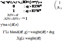
The actual interpolation algorithm calculates the deformations of the grid nodes

for the volume mesh grid nodes xv, i by using the distance dg to the nearest surface of group g. For every coordinate k e {x, y,z} the governing equations are:

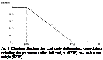
Two new functions have been introduced: the blending function blend( ) and the weighting function weight( -). The weighting function averages the individual group deformations. Because its limit for ds —r 0 is infinity, it needs a cut-off value I / v7£ for numerical reasons.

The blending function is sketched in figure 2. With its group-parameters RZWg (Radius Zero Weight) and RFWg (Radius Full Weight) it is controlling the deform­ation of the grid nodes. If a grid node is close to a boundary of group g with a distance less than RFWg, it will move approximately like the boundary. This func­tionality can be used to conserve the sensitive boundary layer part of a grid. Farther away from the boundary with a distance dg > RZWg the deformation is zero.

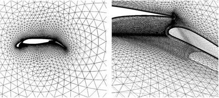
(a) Overall view (b) Zoom view Fig. 3 2d test case, wing including flap and slat. Each of the 3 parts is an independent deform­ation group and only the flap has input values unequal to zero (undeformed: black, deformed: grey)

An example for independently deforming groups can be seen in figure 3. It shows that the surface mesh of the rigid main wing body is not affected by the deformation of the nearby moving flap. The radius zero weight can be recognized in figure 3(a), too.

The algorithm is also described shortly in [6]. This paper also provides test cases showing the usefulness of the presented group-weighting approach and the quality conserving capability of the methodology.

Several different boundary type dependent algorithms have been developed to simplify the usage of standard cases often applied to CFD meshes for aircrafts:

• Standard Boundary Type. This is handled as described above. Deformation vec­tors have to be provided for this surface type.

• No-Normal-Movement Boundary Type. All surface points on this boundary are allowed to slide on the surface. The movement in surface normal direction is suppressed. It’s used for example for symmetry planes.

• Far-field Boundary Type. Here the deformation is set to zero.

• Attached Group Boundary Type. This treatment conserves the shape of an at­tached device, e. g. an engine mounted on a deforming wing.