COMBINED MOMENTUM AND BLADE ELEMENT THEORY WITH EMPIRICAL CORRECTIONS

1. Given: Rotor geometry—number of blades, radius, chord, twist, cutout, airfoil data; and test conditions—tip speed, atmospheric density, speed of sound.

2. Select a finite number of blade elements (at least five but not more than fifteen).

3. At the boundary between each blade element, tabulate: nondimen – sional blade station r/R nondimensional chord, c/R local Mach number, M — (f/RJKnRJ/FsJ; slope of lift curve, a =/(M), per radian, from airfoil data such as Figure 1.10; local twist, A0.

4. Choose collective pitch, 90; tabulate pitch at boundary between each blade element:

9 = 90 + Л9 – aL0

Note: Choose minimum value of 0O so that 0 is always positive.

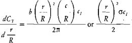
5. Calculate the local inflow angle

32Л0 — R

b_ Clr

1 + 1 +

r 16л — R

or, for a constant chord blade:

Note: 0 and a are in radian units in this equation.

6. Calculate the local angle of attack:

A

a = 0 — tan-1 — degrees

л Ы

7. Using curves of airfoil data such as Figure 1.10 or equations such as those developed in Chapter 6, tabulate ct and cd for the local angle of attack and Mach number. Note: If airfoil data synthesized from whirl tower or model rig test results are being used, they already include the compressibility tip relief effect. If, on the other hand, airfoil data from a two-dimensional wind tunnel are being used, the tip relief may be accounted for by reducing the local Mach number of the outer 10% of the blade by the increment corresponding to the thickness ratio of the tip airfoil from Figure 3.38 of Chapter 3.

8.

Compute the running thrust loading:

9.

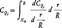
Integrate either graphically or numerically to obtain the thrust coefficient without tip loss:

10. Calculate tip loss factor:

B= 1

Note: All the airfoil data tabulated in Chapter 6 as originating from whirl tower or model rig test results were synthesized from two-bladed
rotors with the assumption that the effective radius was constant at

0. 97 R. If these airfoil data are used, the same assumption should be made, at least in the range of thrust coefficients used in the tests. A study using the airfoil data from reference 1.1 indicates that satisfactory correlation is obtained for a wide range of rotor parameters if the following effective radius equations are used:

for Cr < 0.006

11.

Calculate the corrected thrust coefficient using either graphical or numerical integration:

12.

Compute the running profile torque loading:

13.

Integrate for the profile torque coefficient:

14.

Compute the running induced torque loading:

15.

Integrate for the induced torque coefficient:

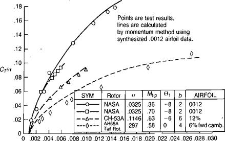
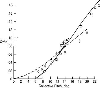
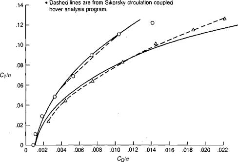
The method has been used with the synthesized 0012 airfoil characteristics on several rotors for which whirl tower data have been published. Figure 1.42 shows correlation with the NACA two-bladed, low-solidity rotor of reference 1.1; the moderate solidity CH-53A rotor of reference 1.5; and the high solidity AH – 56A tail rotor of reference 1.24. It may be seen that the correlation is satisfactory both in power and in collective pitch. Figure 1.43 presents test results from two Sikorsky whirl tower tests, one for a main rotor and the other for a tail rotor. The test points are compared with the results of two calculation schemes: the momentum-blade element method of this book; and the Circulation Coupled Hover Analysis Program (CCHAP) described in reference 1.25. It may be seen that the momentum-blade element method gives satisfactory correlation except at very high thrust levels and is therefore adequate for most hover calculations of a practical, engineering nature. Figure 1.44 shows the performance of the main and tail rotors of the example helicopter calculated by the simple method, and

CqI(j

FIGURE 1.42 Correlation of Test Results with Calculated Results

Source: Carpenter, “Lift and Profile-Drag Characteristics of a NACA 0012 Airfoil Section as Derived from Measured Helicopter-Rotor Hovering Performance,” NACA TN 4357, 1958; Landgrebe, “An Analytical and Experimental Investigation of Helicopter Rotor Hover Performance and Wake Geometry Characteristics," USAAMRDLTR 71-24, 1971; Johnston & Cook, "AH-56A Vehicle Development,” AHS 27th Forum, 1971.

Symb.	Rotor	a	Mtip	©1	b	Airfoil	Ref.
0	"Baseline" main rotor	.0894	.523	-9.25	6	0012	1.40
A	Tail rotor	.20	.63	-8	4	0012	1:24

• Points are test results. • Solid lines are from momentum method of this book.

FIGURE 1.43 Correlation of Prediction Methods with Sikorsky Whirl Tower Test Data

Source: Rorke, "Hover Performance Tests of Full Scale Variable Geometry Rotors,” NASA CR 2713, 1976; Landgrebe, “Aerodynamic Theory for Advanced Rotorcraft” JAHS 22-2, 1977.

Figure 1.45 shows the various elements of the calculation for the main rotor at a collective pitch of 17.5°.