LONGITUDINAL CHARACTERISTICS OF A STOL AIRPLANE
The curves of Figs. 9.4 and 9.5 show that the characteristic modes of an airplane vary markedly with speed, i. e. with the equilibrium weight coefficient CWe. In particular, the two characteristic periods begin to approach one another as CWe becomes large. It is of interest to explore this range more fully by considering an STOL airplane, operating in the “powered-lift” region for which Cw may be much larger. To this end the data given in ref. 7.11, part of which is shown in Fig. 7.6, has been used to obtain a representative set of coefficients for 2.0 < Cff( < 5.0. The flight condition assumed is horizontal steady flight, so that C% = 0 (see Fig. 7.66). (The particular data used from the reference was that for the aircraft with a large tail in the high position, it = 0, and df = 45°.) From the given curves, and from cross-plots of the coefficients CL, CD, and Cm vs. GT at constant a, the data in Table 9.3 was derived for the equilibrium condition. Smooth curves were used for interpolation. Since this is not a tilt-wing airplane, aT is not large in the eases considered, and has been assumed to be zero.
Basic Data for STOL Airplane
|
Table 9.3
|
%hn = .30 – CmJCLx
 |
Since aeroelastic and compressibility effects are negligible at the low speeds of STOL flight the required speed derivatives are given by (see Table 7.1)
For a propeller-driven airplane, the value of CTy is given by (7.8,6), and an examination of the data on ц for a typical constant-speed propeller at low speedf showed that (VJrje)(drildV)e is close to unity. Hence we have used GTy = —2GTe in this example.
Using the formulae of Table 7.1, the following estimates were made of the q and ot derivatives:
CLq=U, Gm<i = —17.9, = 5.5, <^=-13
Finally the following inertial and geometric characteristics were assumed:
W = 40,000 lb, S = 1000 ft2, A = 5.42, c = 13.60 ft H = 76.8, ly = 385, h = .30
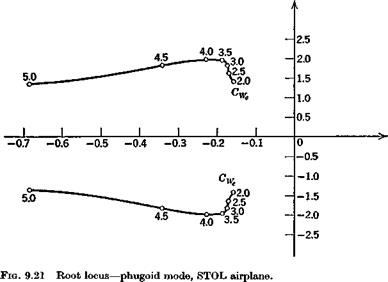
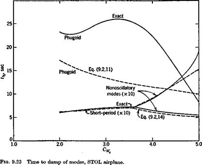
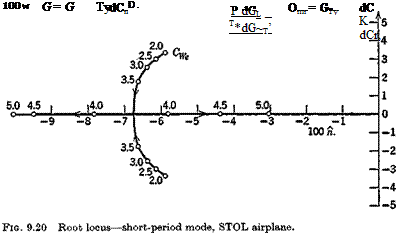
With the above data, the coefficients of the system matrix (9.1,1) were evaluated, and its eigenvalues and eigenvectors calculated. The main results are shown on Figs. 9.20 to 9.24. Figures 9.20 and 9.21 show the loci of the roots as Gw varies between 2 and 5. The effect of GWe is seen to be large on both modes, the short-period mode becoming nonoscillatory at a value of Cw somewhat greater than 3.5, and the damping of the phugoid increasing
f The De Havilland Buffalo airplane. .
|
|
|
|
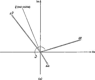
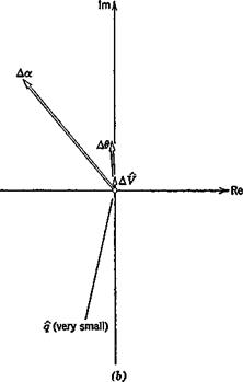
Fig. 9.24 (a) STOL airplane, vector diagram of phugoid mode. Gw — 3.5. (6) Short- period mode. GWe = 3.5. |
|
Fig. 9.24 (Grntd.) |
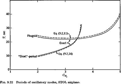
rapidly at the same time. Figure 9.22 shows the two periods, and that they actually cross over at Cw == 3.4. The concept of the phugoid as a “long” period oscillation is evidently not applicable in this situation! The approximations (9.2,11) to the phugoid, and (9.2,14) to the pitching mode are also shown for comparison. It is seen that they give the two periods quite well, and that (9.2,14) also depicts quite accurately the damping of the pitching oscillation and of the two nonperiodic modes into which it degenerates at high GWf. The phugoid damping, however, is not at all well predicted by the approximate solution, and (9.2,9) gives even larger discrepancies for both period and damping. Figure 9.23 shows the damping times for the modes, and they are all seen to be heavily damped over the whole range.
The eigenvectors for the two modes are shown on Fig. 9.24 for GWe = 3.5, the condition of nearly equal periods. The relative configurations of the vectors are seen to be quite similar to those for the jet transport at Gw =1.8 (Fig. 9.6), but the magnitudes of Да in the phugoid, and Д^ in the short – period mode are appreciably larger.
|
From the system theory presented in Chapter 3 we see that it is convenient to classify vehicle motion according to whether it is free or forced. Chapter 9 was devoted to a discussion of a number of examples of the former, and in this chapter we give some illustrations of the latter. The particular cases studied here are those in which the motion results from nonautonomous actuation of the controls. That is, we exclude those in which the controls are moved in response to the vehicle motion in accordance with a prescribed law, as by an autopilot. Such motions are the subject matter of Chapter 11. We should recall as well that for linear/invariant systems (Sec. 3.4) there is really only one fundamental response problem The impulse response, the step response, and the frequency response are all explicitly related, and the convolution theorem (3.4,41) and (3.4,43) enables the response to any arbitrary control variation to he calculated from a knowledge of either the impulse response or the step response.
In the examples that follow, we consider the response of an airplane to actuation of its principal controls, the throttle and the three aerodynamic control surfaces. The examples include both step and frequency response, and both linear and nonlinear cases.
As shown in Chapter 3, the basic item needed for computing frequency
response, and for formulating response problems analytically is the transfer function that relates the relevant responses and inputs. In the present context the input is the control vector. The required transfer functions can be found either from the standard first-order form of the differential equations of motion, in which case they are given by (3.2,23), or from the Laplace transforms of the equations (5.11,8 to 10) or (5.14,1 to 3). There is an essential theoretical difference between the two methods, since the former implies the representation of the aerodynamic forces by means of aerodynamic derivatives, and the latter allows (but does not require) the use of exact linear aerodynamics (see Sec. 5.11). Practically, there is only a difference between the responses calculated by the two approaches when the aerodynamic control surfaces are moved very rapidly.


